Code
import tensorflow as tf
import numpy as np
import pandas as pd
import matplotlib.pyplot as plt

plt.rcParams['figure.figsize'] = (10, 8)kakamana
April 7, 2023
This chapter focuses on building two-input networks using categorical embeddings for high-cardinality data, shared layers for re-usable building blocks, and merged layers for joining multiple inputs together. You will have the foundational building blocks for designing neural networks with complex data flows at the end of this chapter.
This Two Input Networks Using Categorical Embeddings, Shared Layers, and Merge Layers is part of [Datacamp course: Advanced Deep Learning with Keras] You will learn how to use the versatile Keras functional API to solve a variety of problems. The course will begin with simple, multi-layer dense networks (also known as multi-layer perceptrons) and progress to more sophisticated architectures. This course will cover how to construct models with multiple inputs and a single output, as well as how to share weights between layers in a model. Additionally, we will discuss advanced topics such as category embeddings and multiple output networks. This course will teach you how to train a network that performs both classification and regression.
This is my learning experience of data science through DataCamp. These repository contributions are part of my learning journey through my graduate program masters of applied data sciences (MADS) at University Of Michigan, DeepLearning.AI, Coursera & DataCamp. You can find my similar articles & more stories at my medium & LinkedIn profile. I am available at kaggle & github blogs & github repos. Thank you for your motivation, support & valuable feedback.
These include projects, coursework & notebook which I learned through my data science journey. They are created for reproducible & future reference purpose only. All source code, slides or screenshot are intellactual property of respective content authors. If you find these contents beneficial, kindly consider learning subscription from DeepLearning.AI Subscription, Coursera, DataCamp

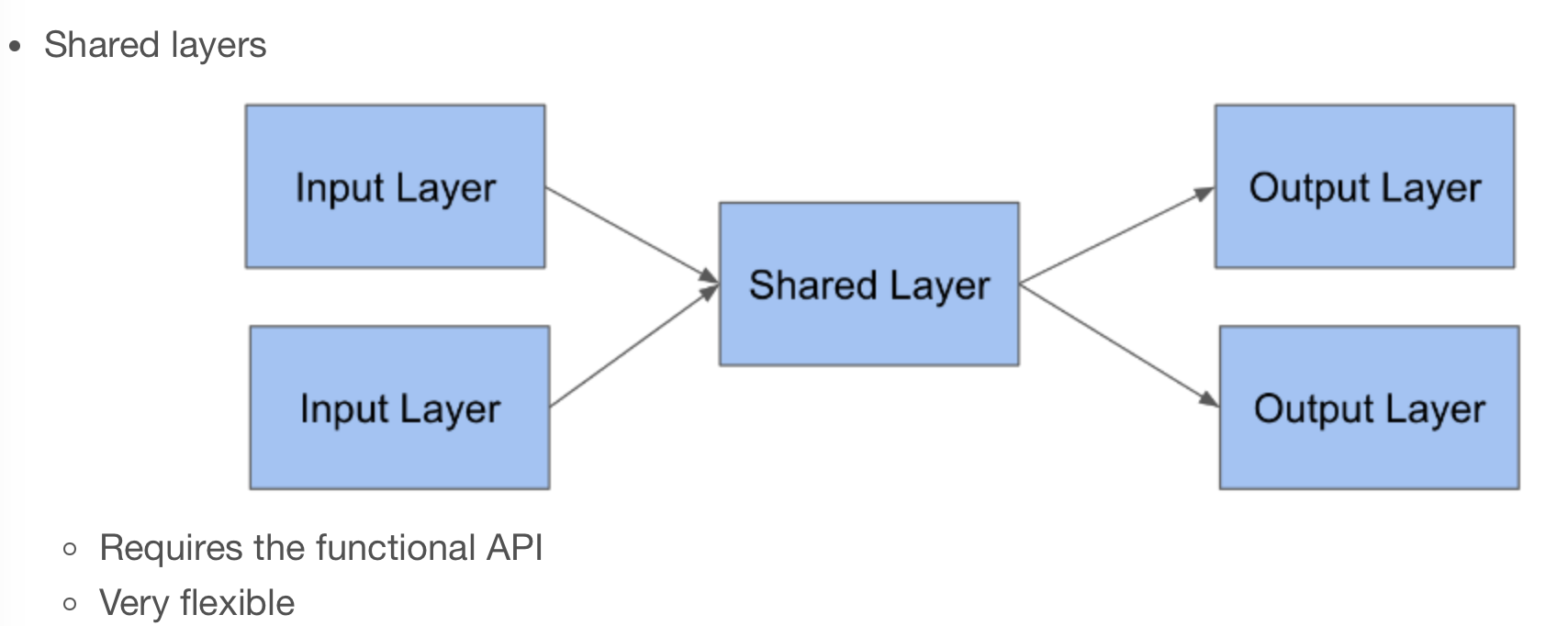
Shared layers allow a model to use the same weight matrix for multiple steps. In this exercise, you will build a “team strength” layer that represents each team by a single number. You will use this number for both teams in the model. The model will learn a number for each team that works well both when the team is team_1 and when the team is team_2 in the input data.
| season | team_1 | team_2 | home | score_diff | score_1 | score_2 | won | |
|---|---|---|---|---|---|---|---|---|
| 0 | 1985 | 3745 | 6664 | 0 | 17 | 81 | 64 | 1 |
| 1 | 1985 | 126 | 7493 | 1 | 7 | 77 | 70 | 1 |
| 2 | 1985 | 288 | 3593 | 1 | 7 | 63 | 56 | 1 |
| 3 | 1985 | 1846 | 9881 | 1 | 16 | 70 | 54 | 1 |
| 4 | 1985 | 2675 | 10298 | 1 | 12 | 86 | 74 | 1 |
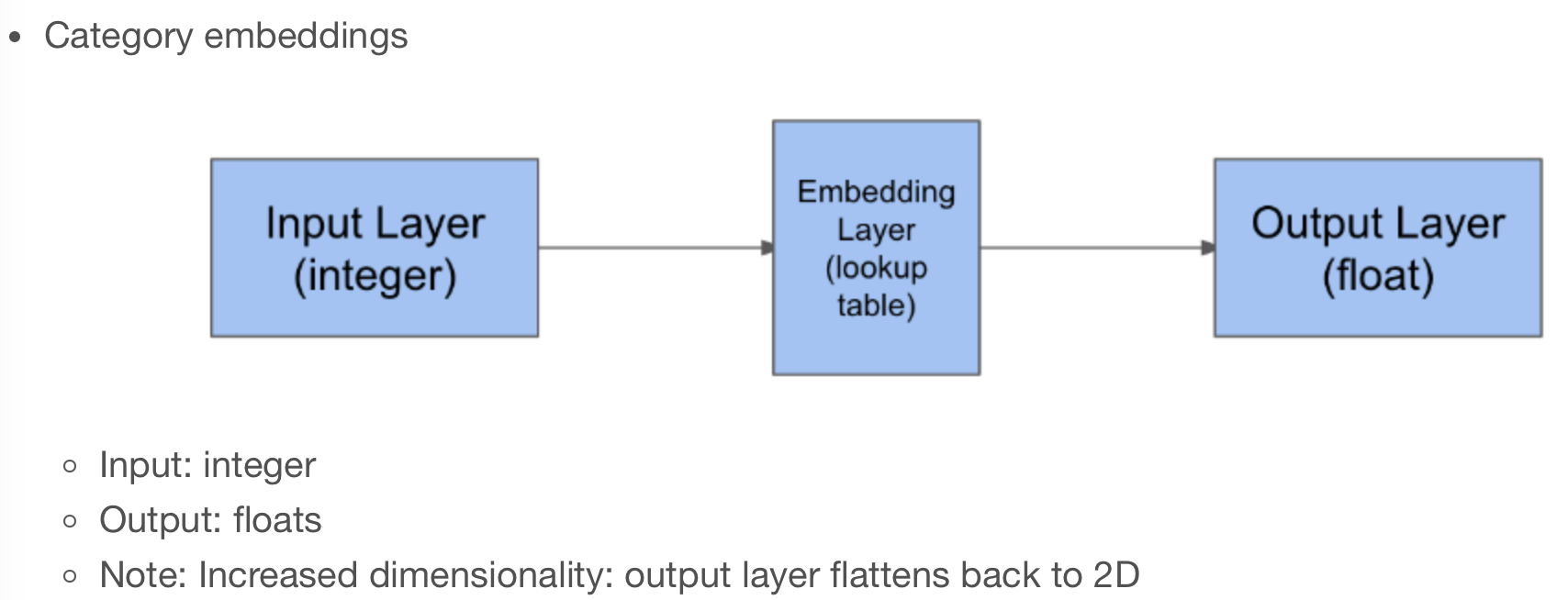
The team strength lookup has three components: an input, an embedding layer, and a flatten layer that creates the output.
If you wrap these three layers in a model with an input and output, you can re-use that stack of three layers at multiple places.
Note again that the weights for all three layers will be shared everywhere we use them.
from tensorflow.keras.layers import Input, Flatten
from tensorflow.keras.models import Model

# Create an input layer for the team ID
teamid_in = Input(shape=(1, ))

# Lookup the input in the team strength embedding layer
strength_lookup = team_lookup(teamid_in)

# Flatten the output
strength_lookup_flat = Flatten()(strength_lookup)

# Combine the operations into a single, re-usable model
team_strength_model = Model(teamid_in, strength_lookup_flat, name='Team-Strength-Model')
Metal device set to: Apple M2 Pro
In this exercise, you will define two input layers for the two teams in your model. This allows you to specify later in the model how the data from each team will be used differently.
Now that you have a team strength model and an input layer for each team, you can lookup the team inputs in the shared team strength model. The two inputs will share the same weights.
In this dataset, you have 10,888 unique teams. You want to learn a strength rating for each team, such that if any pair of teams plays each other, you can predict the score, even if those two teams have never played before. Furthermore, you want the strength rating to be the same, regardless of whether the team is the home team or the away team.
Now that you’ve looked up how “strong” each team is, subtract the team strengths to determine which team is expected to win the game.
This is a bit like the seeds that the tournament committee uses, which are also a measure of team strength. But rather than using seed differences to predict score differences, you’ll use the difference of your own team strength model to predict score differences.
The subtract layer will combine the weights from the two layers by subtracting them.
Now that you have your two inputs (team id 1 and team id 2) and output (score difference), you can wrap them up in a model so you can use it later for fitting to data and evaluating on new data
Fit the model to the regular season training data Now that you’ve defined a complete team strength model, you can fit it to the basketball data! Since your model has two inputs now, you need to pass the input data as a list.
input_1 = games_season['team_1']

# Get the team_2 column from the regular season data
input_2 = games_season['team_2']

# Fit the model to input 1 and 2, using score diff as a target
model.fit([input_1, input_2], games_season['score_diff'], epochs=1, batch_size=2048, validation_split=0.1, verbose=True);
138/138 [==============================] - 1s 6ms/step - loss: 12.0968 - val_loss: 11.8210In this exercise, you will evaluate the model on this new dataset. This evaluation will tell you how well you can predict the tournament games, based on a model trained with the regular season data. This is interesting because many teams play each other in the tournament that did not play in the regular season, so this is a very good check that your model is not overfitting.
| season | team_1 | team_2 | home | seed_diff | score_diff | score_1 | score_2 | won | |
|---|---|---|---|---|---|---|---|---|---|
| 0 | 1985 | 288 | 73 | 0 | -3 | -9 | 41 | 50 | 0 |
| 1 | 1985 | 5929 | 73 | 0 | 4 | 6 | 61 | 55 | 1 |
| 2 | 1985 | 9884 | 73 | 0 | 5 | -4 | 59 | 63 | 0 |
| 3 | 1985 | 73 | 288 | 0 | 3 | 9 | 50 | 41 | 1 |
| 4 | 1985 | 3920 | 410 | 0 | 1 | -9 | 54 | 63 | 0 |