Code
# Import seaborn with alias sns
import pandas as pd
import seaborn as sns
import numpy as np

# Import matplotlib.pyplot with alias plt
import matplotlib.pyplot as pltIt’s time to get hands-on and perform the four random sampling methods in Python: simple, systematic, stratified, and cluster.
This Sampling Methods is part of Datacamp course: Introduction to sampling
This is my learning experience of data science through DataCamp
# Import seaborn with alias sns
import pandas as pd
import seaborn as sns
import numpy as np
# Import matplotlib.pyplot with alias plt
import matplotlib.pyplot as pltAlthough there are several sampling methods such as: * Simple random sampling * Systematic random sampling * Stratified & weight random sampling * Cluster sampling
attrition_pop=pd.read_feather('dataset/attrition.feather')
attrition_pop.head()| Age | Attrition | BusinessTravel | DailyRate | Department | DistanceFromHome | Education | EducationField | EnvironmentSatisfaction | Gender | ... | PerformanceRating | RelationshipSatisfaction | StockOptionLevel | TotalWorkingYears | TrainingTimesLastYear | WorkLifeBalance | YearsAtCompany | YearsInCurrentRole | YearsSinceLastPromotion | YearsWithCurrManager | |
|---|---|---|---|---|---|---|---|---|---|---|---|---|---|---|---|---|---|---|---|---|---|
| 0 | 21 | 0.0 | Travel_Rarely | 391 | Research_Development | 15 | College | Life_Sciences | High | Male | ... | Excellent | Very_High | 0 | 0 | 6 | Better | 0 | 0 | 0 | 0 |
| 1 | 19 | 1.0 | Travel_Rarely | 528 | Sales | 22 | Below_College | Marketing | Very_High | Male | ... | Excellent | Very_High | 0 | 0 | 2 | Good | 0 | 0 | 0 | 0 |
| 2 | 18 | 1.0 | Travel_Rarely | 230 | Research_Development | 3 | Bachelor | Life_Sciences | High | Male | ... | Excellent | High | 0 | 0 | 2 | Better | 0 | 0 | 0 | 0 |
| 3 | 18 | 0.0 | Travel_Rarely | 812 | Sales | 10 | Bachelor | Medical | Very_High | Female | ... | Excellent | Low | 0 | 0 | 2 | Better | 0 | 0 | 0 | 0 |
| 4 | 18 | 1.0 | Travel_Frequently | 1306 | Sales | 5 | Bachelor | Marketing | Medium | Male | ... | Excellent | Very_High | 0 | 0 | 3 | Better | 0 | 0 | 0 | 0 |
5 rows × 31 columns
# Sample 70 rows using simple random sampling and set the seed
attrition_samp = attrition_pop.sample(n=70, random_state=18900217)

# Print the sample
print(attrition_samp)
Age Attrition BusinessTravel DailyRate Department \
1134 35 0.0 Travel_Rarely 583 Research_Development
1150 52 0.0 Non-Travel 585 Sales
531 33 0.0 Travel_Rarely 931 Research_Development
395 31 0.0 Travel_Rarely 1332 Research_Development
392 29 0.0 Travel_Rarely 942 Research_Development
... ... ... ... ... ...
361 27 0.0 Travel_Frequently 1410 Sales
1180 36 0.0 Travel_Rarely 530 Sales
230 26 0.0 Travel_Rarely 1443 Sales
211 29 0.0 Travel_Frequently 410 Research_Development
890 30 0.0 Travel_Frequently 1312 Research_Development
DistanceFromHome Education EducationField \
1134 25 Master Medical
1150 29 Master Life_Sciences
531 14 Bachelor Medical
395 11 College Medical
392 15 Below_College Life_Sciences
... ... ... ...
361 3 Below_College Medical
1180 2 Master Life_Sciences
230 23 Bachelor Marketing
211 2 Below_College Life_Sciences
890 2 Master Technical_Degree
EnvironmentSatisfaction Gender ... PerformanceRating \
1134 High Female ... Excellent
1150 Low Male ... Excellent
531 Very_High Female ... Excellent
395 High Male ... Excellent
392 Medium Female ... Excellent
... ... ... ... ...
361 Very_High Female ... Outstanding
1180 High Female ... Excellent
230 High Female ... Excellent
211 Very_High Female ... Excellent
890 Very_High Female ... Excellent
RelationshipSatisfaction StockOptionLevel TotalWorkingYears \
1134 High 1 16
1150 Medium 2 16
531 Very_High 1 8
395 Very_High 0 6
392 Low 1 6
... ... ... ...
361 Medium 2 6
1180 High 0 17
230 High 1 5
211 High 3 4
890 Very_High 0 10
TrainingTimesLastYear WorkLifeBalance YearsAtCompany \
1134 3 Good 16
1150 3 Good 9
531 5 Better 8
395 2 Good 6
392 2 Good 5
... ... ... ...
361 3 Better 6
1180 2 Good 13
230 2 Good 2
211 3 Better 3
890 2 Better 9
YearsInCurrentRole YearsSinceLastPromotion YearsWithCurrManager
1134 10 10 1
1150 8 0 0
531 7 1 6
395 5 0 1
392 4 1 3
... ... ... ...
361 5 0 4
1180 7 6 7
230 2 0 0
211 2 0 2
890 7 0 7
[70 rows x 31 columns]# Set the sample size to 70
sample_size = 70
# Calculate the population size from attrition_pop
pop_size = len(attrition_pop)
# Calculate the interval
interval = pop_size // sample_size
# Systematically sample 70 rows
attrition_sys_samp = attrition_pop.iloc[::interval]
# Print the sample
print(attrition_sys_samp) Age Attrition BusinessTravel DailyRate Department \
0 21 0.0 Travel_Rarely 391 Research_Development
21 19 0.0 Travel_Rarely 1181 Research_Development
42 45 0.0 Travel_Rarely 252 Research_Development
63 23 0.0 Travel_Rarely 373 Research_Development
84 30 1.0 Travel_Rarely 945 Sales
... ... ... ... ... ...
1365 48 0.0 Travel_Rarely 715 Research_Development
1386 48 0.0 Travel_Rarely 1355 Research_Development
1407 50 0.0 Travel_Rarely 989 Research_Development
1428 50 0.0 Non-Travel 881 Research_Development
1449 52 0.0 Travel_Rarely 699 Research_Development
DistanceFromHome Education EducationField EnvironmentSatisfaction \
0 15 College Life_Sciences High
21 3 Below_College Medical Medium
42 2 Bachelor Life_Sciences Medium
63 1 College Life_Sciences Very_High
84 9 Bachelor Medical Medium
... ... ... ... ...
1365 1 Bachelor Life_Sciences Very_High
1386 4 Master Life_Sciences High
1407 7 College Medical Medium
1428 2 Master Life_Sciences Low
1449 1 Master Life_Sciences High
Gender ... PerformanceRating RelationshipSatisfaction \
0 Male ... Excellent Very_High
21 Female ... Excellent Very_High
42 Female ... Excellent Very_High
63 Male ... Outstanding Very_High
84 Male ... Excellent High
... ... ... ... ...
1365 Male ... Excellent High
1386 Male ... Excellent Medium
1407 Female ... Excellent Very_High
1428 Male ... Excellent Very_High
1449 Male ... Excellent Low
StockOptionLevel TotalWorkingYears TrainingTimesLastYear \
0 0 0 6
21 0 1 3
42 0 1 3
63 1 1 2
84 0 1 3
... ... ... ...
1365 0 25 3
1386 0 27 3
1407 1 29 2
1428 1 31 3
1449 1 34 5
WorkLifeBalance YearsAtCompany YearsInCurrentRole \
0 Better 0 0
21 Better 1 0
42 Better 1 0
63 Better 1 0
84 Good 1 0
... ... ... ...
1365 Best 1 0
1386 Better 15 11
1407 Good 27 3
1428 Better 31 6
1449 Better 33 18
YearsSinceLastPromotion YearsWithCurrManager
0 0 0
21 0 0
42 0 0
63 0 1
84 0 0
... ... ...
1365 0 0
1386 4 8
1407 13 8
1428 14 7
1449 11 9
[70 rows x 31 columns]In the case of systematic sampling, there is a problem: if the data has been sorted or there is a pattern or meaning behind the row order, then the resulting sample may not be representative of the entire population. If the rows are shuffled, the problem can be solved, but then systematic sampling becomes equivalent to simple random sampling.
# Add an index column to attrition_pop
attrition_pop_id = attrition_pop.reset_index()

# Plot YearsAtCompany vs. index for attrition_pop_id
attrition_pop_id.plot(x='index',y='YearsAtCompany',kind='scatter')
plt.show()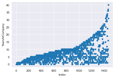
# Shuffle the rows of attrition_pop
attrition_shuffled = attrition_pop.sample(frac=1)

# Reset the row indexes and create an index column
attrition_shuffled = attrition_shuffled.reset_index(drop=True).reset_index()

# Plot YearsAtCompany vs. index for attrition_shuffled
attrition_shuffled.plot(x='index',y='YearsAtCompany',kind='scatter')
plt.show()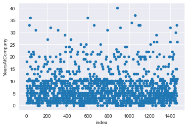
Stratified sampling is a technique that allows us to sample a population that contains subgroups
A close relative of stratified sampling that provides even more flexibility is weighted random sampling. In this variant, we create a column of weights that adjust the relative probability of sampling each row.
You may need to carefully control the counts of each subgroup within the population if you are interested in subgroups within the population. As a result of proportional stratified sampling, the subgroup sizes within the sample are representative of the subgroup sizes within the population as a whole.
# Proportion of employees by Education level
education_counts_pop = attrition_pop['Education'].value_counts(normalize=True)

# Print education_counts_pop
print(education_counts_pop)
Bachelor 0.389116
Master 0.270748
College 0.191837
Below_College 0.115646
Doctor 0.032653
Name: Education, dtype: float64# Proportional stratified sampling for 40% of each Education group
attrition_strat = attrition_pop.groupby('Education').sample(frac=0.4, random_state=2022)
# Print the sample
print(attrition_strat) Age Attrition BusinessTravel DailyRate Department \
1191 53 0.0 Travel_Rarely 238 Sales
407 29 0.0 Travel_Frequently 995 Research_Development
1233 59 0.0 Travel_Frequently 1225 Sales
366 37 0.0 Travel_Rarely 571 Research_Development
702 31 0.0 Travel_Frequently 163 Research_Development
... ... ... ... ... ...
733 38 0.0 Travel_Frequently 653 Research_Development
1061 44 0.0 Travel_Frequently 602 Human_Resources
1307 41 0.0 Travel_Rarely 1276 Sales
1060 33 0.0 Travel_Rarely 516 Research_Development
177 29 0.0 Travel_Rarely 738 Research_Development
DistanceFromHome Education EducationField \
1191 1 Below_College Medical
407 2 Below_College Life_Sciences
1233 1 Below_College Life_Sciences
366 10 Below_College Life_Sciences
702 24 Below_College Technical_Degree
... ... ... ...
733 29 Doctor Life_Sciences
1061 1 Doctor Human_Resources
1307 2 Doctor Life_Sciences
1060 8 Doctor Life_Sciences
177 9 Doctor Other
EnvironmentSatisfaction Gender ... PerformanceRating \
1191 Very_High Female ... Outstanding
407 Low Male ... Excellent
1233 Low Female ... Excellent
366 Very_High Female ... Excellent
702 Very_High Female ... Outstanding
... ... ... ... ...
733 Very_High Female ... Excellent
1061 Low Male ... Excellent
1307 Medium Female ... Excellent
1060 Very_High Male ... Excellent
177 Medium Male ... Excellent
RelationshipSatisfaction StockOptionLevel TotalWorkingYears \
1191 Very_High 0 18
407 Very_High 1 6
1233 Very_High 0 20
366 Medium 2 6
702 Very_High 0 9
... ... ... ...
733 Very_High 0 10
1061 High 0 14
1307 Medium 1 22
1060 Low 0 14
177 High 0 4
TrainingTimesLastYear WorkLifeBalance YearsAtCompany \
1191 2 Best 14
407 0 Best 6
1233 2 Good 4
366 3 Good 5
702 3 Good 5
... ... ... ...
733 2 Better 10
1061 3 Better 10
1307 2 Better 18
1060 6 Better 0
177 2 Better 3
YearsInCurrentRole YearsSinceLastPromotion YearsWithCurrManager
1191 7 8 10
407 4 1 3
1233 3 1 3
366 3 4 3
702 4 1 4
... ... ... ...
733 3 9 9
1061 7 0 2
1307 16 11 8
1060 0 0 0
177 2 2 2
[588 rows x 31 columns]# Calculate the Education level proportions from attrition_strat
education_counts_strat = attrition_strat['Education'].value_counts(normalize=True)
# Print education_counts_strat
print(education_counts_strat)
print('\nBy grouping then sampling, the size of each group in the sample is representative of the size of the sample in the population.')Bachelor 0.389456
Master 0.270408
College 0.192177
Below_College 0.115646
Doctor 0.032313
Name: Education, dtype: float64
By grouping then sampling, the size of each group in the sample is representative of the size of the sample in the population.When one subgroup is larger than another in the population, but you do not want to factor this difference into your analysis, you can use equal counts stratified sampling to generate samples in which each subgroup has the same amount of data.
# Get 30 employees from each Education group
attrition_eq = attrition_pop.groupby('Education').sample(n=30, random_state=2022)

# Print the sample
print(attrition_eq)
Age Attrition BusinessTravel DailyRate Department \
1191 53 0.0 Travel_Rarely 238 Sales
407 29 0.0 Travel_Frequently 995 Research_Development
1233 59 0.0 Travel_Frequently 1225 Sales
366 37 0.0 Travel_Rarely 571 Research_Development
702 31 0.0 Travel_Frequently 163 Research_Development
... ... ... ... ... ...
774 33 0.0 Travel_Rarely 922 Research_Development
869 45 0.0 Travel_Rarely 1015 Research_Development
530 32 0.0 Travel_Rarely 120 Research_Development
1049 48 0.0 Travel_Rarely 163 Sales
350 29 1.0 Travel_Rarely 408 Research_Development
DistanceFromHome Education EducationField \
1191 1 Below_College Medical
407 2 Below_College Life_Sciences
1233 1 Below_College Life_Sciences
366 10 Below_College Life_Sciences
702 24 Below_College Technical_Degree
... ... ... ...
774 1 Doctor Medical
869 5 Doctor Medical
530 6 Doctor Life_Sciences
1049 2 Doctor Marketing
350 25 Doctor Technical_Degree
EnvironmentSatisfaction Gender ... PerformanceRating \
1191 Very_High Female ... Outstanding
407 Low Male ... Excellent
1233 Low Female ... Excellent
366 Very_High Female ... Excellent
702 Very_High Female ... Outstanding
... ... ... ... ...
774 Low Female ... Excellent
869 High Female ... Excellent
530 High Male ... Outstanding
1049 Medium Female ... Excellent
350 High Female ... Excellent
RelationshipSatisfaction StockOptionLevel TotalWorkingYears \
1191 Very_High 0 18
407 Very_High 1 6
1233 Very_High 0 20
366 Medium 2 6
702 Very_High 0 9
... ... ... ...
774 High 1 10
869 Low 0 10
530 Low 0 8
1049 Low 1 14
350 Medium 0 6
TrainingTimesLastYear WorkLifeBalance YearsAtCompany \
1191 2 Best 14
407 0 Best 6
1233 2 Good 4
366 3 Good 5
702 3 Good 5
... ... ... ...
774 2 Better 6
869 3 Better 10
530 2 Better 5
1049 2 Better 9
350 2 Best 2
YearsInCurrentRole YearsSinceLastPromotion YearsWithCurrManager
1191 7 8 10
407 4 1 3
1233 3 1 3
366 3 4 3
702 4 1 4
... ... ... ...
774 1 0 5
869 7 1 4
530 4 1 4
1049 7 6 7
350 2 1 1
[150 rows x 31 columns]# Get the proportions from attrition_eq
education_counts_eq = attrition_eq['Education'].value_counts(normalize=True)
# Print the results
print(education_counts_eq)Below_College 0.2
College 0.2
Bachelor 0.2
Master 0.2
Doctor 0.2
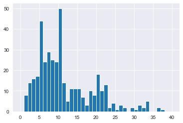
Name: Education, dtype: float64The stratified sampling method determines the probability of picking rows from your dataset based on the subgroups within your dataset. A generalization of this is weighted sampling, which allows you to specify rules regarding the probability of selecting rows at the row level. A row’s probability of being selected is proportional to its weight value.
# Plot YearsAtCompany from attrition_pop as a histogram
attrition_pop['YearsAtCompany'].hist(bins=np.arange(0,41,1))
plt.show()
# Sample 400 employees weighted by YearsAtCompany
attrition_weight = attrition_pop.sample(n=400, weights='YearsAtCompany')

# Print the sample
print(attrition_weight)
Age Attrition BusinessTravel DailyRate Department \
853 36 0.0 Travel_Rarely 172 Research_Development
481 34 0.0 Travel_Frequently 618 Research_Development
1148 38 0.0 Travel_Rarely 1321 Sales
1430 51 0.0 Travel_Frequently 237 Sales
517 39 0.0 Travel_Rarely 835 Research_Development
... ... ... ... ... ...
1351 45 0.0 Travel_Rarely 1038 Research_Development
1412 54 0.0 Travel_Rarely 971 Research_Development
1248 47 0.0 Travel_Frequently 1379 Research_Development
1210 36 0.0 Travel_Frequently 688 Research_Development
1328 55 0.0 Travel_Frequently 1091 Research_Development
DistanceFromHome Education EducationField EnvironmentSatisfaction \
853 4 Master Life_Sciences Low
481 3 Below_College Life_Sciences Low
1148 1 Master Life_Sciences Very_High
1430 9 Bachelor Life_Sciences Very_High
517 19 Master Other Very_High
... ... ... ... ...
1351 20 Bachelor Medical Medium
1412 1 Bachelor Medical Very_High
1248 16 Master Medical High
1210 4 College Life_Sciences Very_High
1328 2 Below_College Life_Sciences Very_High
Gender ... PerformanceRating RelationshipSatisfaction \
853 Male ... Excellent High
481 Male ... Excellent High
1148 Male ... Excellent Low
1430 Male ... Outstanding Low
517 Male ... Excellent Medium
... ... ... ... ...
1351 Male ... Excellent Medium
1412 Female ... Excellent Very_High
1248 Male ... Excellent High
1210 Female ... Excellent Medium
1328 Male ... Excellent Medium
StockOptionLevel TotalWorkingYears TrainingTimesLastYear \
853 0 10 2
481 0 7 1
1148 2 16 3
1430 1 31 5
517 3 7 2
... ... ... ...
1351 1 24 2
1412 0 29 3
1248 0 20 3
1210 3 18 3
1328 1 23 4
WorkLifeBalance YearsAtCompany YearsInCurrentRole \
853 Good 10 4
481 Good 6 2
1148 Better 15 13
1430 Good 29 10
517 Better 2 2
... ... ... ...
1351 Better 7 7
1412 Good 20 7
1248 Best 19 10
1210 Better 4 2
1328 Better 3 2
YearsSinceLastPromotion YearsWithCurrManager
853 1 8
481 0 4
1148 5 8
1430 11 10
517 2 2
... ... ...
1351 0 7
1412 12 7
1248 2 7
1210 0 2
1328 1 2
[400 rows x 31 columns]# Plot YearsAtCompany from attrition_weight as a histogram
attrition_weight['YearsAtCompany'].hist(bins=np.arange(0,41,1))
plt.show()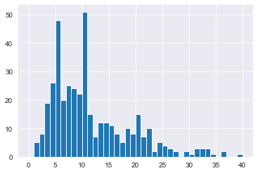
# Plot YearsAtCompany from attrition_pop as a histogram
attrition_pop['YearsAtCompany'].hist(bins=np.arange(0, 41, 1))
plt.show()
# Sample 400 employees weighted by YearsAtCompany
attrition_weight = attrition_pop.sample(n=400, weights="YearsAtCompany")
# Plot YearsAtCompany from attrition_weight as a histogram
attrition_weight['YearsAtCompany'].hist(bins=np.arange(0,41,1))
plt.show()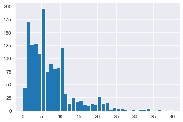
Stratified sampling vs. cluster sampling * Stratified sampling: * Split the population into subgroups * Use simple random sampling on every subgroup * Cluster sampling * Use simple random sampling to pick some subgroups * Use simple random sampling on only those subgroups
import random
# Create a list of unique JobRole values
job_roles_pop = list(attrition_pop['JobRole'].unique())

# Randomly sample four JobRole values
job_roles_samp = random.sample(job_roles_pop,k=4)

# Print the result
print(job_roles_samp)
['Research_Director', 'Sales_Executive', 'Sales_Representative', 'Laboratory_Technician']# Filter for rows where JobRole is in job_roles_samp
jobrole_condition = attrition_pop['JobRole'].isin(job_roles_samp)
attrition_filtered = attrition_pop[jobrole_condition]
# Print the result
print(attrition_filtered) Age Attrition BusinessTravel DailyRate Department \
1 19 1.0 Travel_Rarely 528 Sales
2 18 1.0 Travel_Rarely 230 Research_Development
3 18 0.0 Travel_Rarely 812 Sales
4 18 1.0 Travel_Frequently 1306 Sales
7 18 1.0 Non-Travel 247 Research_Development
... ... ... ... ... ...
1457 55 0.0 Travel_Rarely 692 Research_Development
1458 56 0.0 Travel_Frequently 906 Sales
1459 54 0.0 Travel_Rarely 685 Research_Development
1467 58 0.0 Travel_Rarely 682 Sales
1469 58 1.0 Travel_Rarely 286 Research_Development
DistanceFromHome Education EducationField EnvironmentSatisfaction \
1 22 Below_College Marketing Very_High
2 3 Bachelor Life_Sciences High
3 10 Bachelor Medical Very_High
4 5 Bachelor Marketing Medium
7 8 Below_College Medical High
... ... ... ... ...
1457 14 Master Medical High
1458 6 Bachelor Life_Sciences High
1459 3 Bachelor Life_Sciences Very_High
1467 10 Master Medical Very_High
1469 2 Master Life_Sciences Very_High
Gender ... PerformanceRating RelationshipSatisfaction \
1 Male ... Excellent Very_High
2 Male ... Excellent High
3 Female ... Excellent Low
4 Male ... Excellent Very_High
7 Male ... Excellent Very_High
... ... ... ... ...
1457 Male ... Excellent Very_High
1458 Female ... Excellent Very_High
1459 Male ... Excellent Low
1467 Male ... Excellent High
1469 Male ... Excellent Very_High
StockOptionLevel TotalWorkingYears TrainingTimesLastYear \
1 0 0 2
2 0 0 2
3 0 0 2
4 0 0 3
7 0 0 0
... ... ... ...
1457 0 36 3
1458 3 36 0
1459 0 36 2
1467 0 38 1
1469 0 40 2
WorkLifeBalance YearsAtCompany YearsInCurrentRole \
1 Good 0 0
2 Better 0 0
3 Better 0 0
4 Better 0 0
7 Better 0 0
... ... ... ...
1457 Better 24 15
1458 Good 7 7
1459 Better 10 9
1467 Good 37 10
1469 Better 31 15
YearsSinceLastPromotion YearsWithCurrManager
1 0 0
2 0 0
3 0 0
4 0 0
7 0 0
... ... ...
1457 2 15
1458 7 7
1459 0 9
1467 1 8
1469 13 8
[748 rows x 31 columns]# Remove categories with no rows
attrition_filtered['JobRole'] = attrition_filtered['JobRole'].cat.remove_unused_categories()
# Randomly sample 10 employees from each sampled job role
attrition_clust = attrition_filtered.groupby('JobRole').sample(n=10,random_state=2022)
# Print the sample
print(attrition_clust)
print("\n The two-stage sampling technique gives you control over sampling both between subgroups and within subgroups.") Age Attrition BusinessTravel DailyRate Department \
1124 36 0.0 Travel_Rarely 1396 Research_Development
576 45 0.0 Travel_Rarely 974 Research_Development
995 42 0.0 Travel_Frequently 748 Research_Development
1243 50 0.0 Travel_Rarely 1207 Research_Development
869 45 0.0 Travel_Rarely 1015 Research_Development
599 33 0.0 Travel_Rarely 1099 Research_Development
117 24 0.0 Travel_Rarely 350 Research_Development
472 30 0.0 Travel_Rarely 921 Research_Development
149 27 0.0 Non-Travel 1277 Research_Development
49 20 1.0 Travel_Rarely 129 Research_Development
1302 40 0.0 Travel_Rarely 1416 Research_Development
1126 42 0.0 Travel_Rarely 810 Research_Development
1216 38 0.0 Travel_Rarely 849 Research_Development
1362 43 0.0 Travel_Rarely 982 Research_Development
1327 46 0.0 Travel_Rarely 430 Research_Development
664 27 0.0 Travel_Rarely 269 Research_Development
1284 40 0.0 Travel_Rarely 1308 Research_Development
1440 50 0.0 Travel_Frequently 333 Research_Development
790 36 0.0 Non-Travel 427 Research_Development
1432 55 0.0 Travel_Rarely 1136 Research_Development
941 36 0.0 Travel_Rarely 329 Sales
454 27 0.0 Travel_Frequently 1242 Sales
460 37 0.0 Travel_Rarely 228 Sales
636 45 0.0 Travel_Rarely 1268 Sales
293 33 0.0 Travel_Frequently 430 Sales
976 39 1.0 Travel_Rarely 1162 Sales
813 30 0.0 Travel_Rarely 231 Sales
288 35 1.0 Travel_Frequently 662 Sales
1111 53 1.0 Travel_Rarely 1168 Sales
1075 40 0.0 Travel_Rarely 630 Sales
133 34 1.0 Travel_Frequently 296 Sales
725 36 1.0 Travel_Rarely 1218 Sales
4 18 1.0 Travel_Frequently 1306 Sales
169 41 1.0 Travel_Rarely 1356 Sales
1 19 1.0 Travel_Rarely 528 Sales
48 19 1.0 Travel_Rarely 419 Sales
150 31 0.0 Travel_Frequently 793 Sales
130 21 0.0 Non-Travel 895 Sales
3 18 0.0 Travel_Rarely 812 Sales
99 31 0.0 Travel_Frequently 444 Sales
DistanceFromHome Education EducationField \
1124 5 College Life_Sciences
576 1 Master Medical
995 9 College Medical
1243 28 Below_College Medical
869 5 Doctor Medical
599 4 Master Medical
117 21 College Technical_Degree
472 1 Bachelor Life_Sciences
149 8 Doctor Life_Sciences
49 4 Bachelor Technical_Degree
1302 2 College Medical
1126 23 Doctor Life_Sciences
1216 25 College Life_Sciences
1362 12 Bachelor Life_Sciences
1327 1 Master Medical
664 5 Below_College Technical_Degree
1284 14 Bachelor Medical
1440 22 Doctor Medical
790 8 Bachelor Life_Sciences
1432 1 Master Medical
941 16 Master Marketing
454 20 Bachelor Life_Sciences
460 6 Master Medical
636 4 College Life_Sciences
293 7 Bachelor Medical
976 3 College Medical
813 8 College Other
288 18 Master Marketing
1111 24 Master Life_Sciences
1075 4 Master Marketing
133 6 College Marketing
725 9 Master Life_Sciences
4 5 Bachelor Marketing
169 20 College Marketing
1 22 Below_College Marketing
48 21 Bachelor Other
150 20 Bachelor Life_Sciences
130 9 College Medical
3 10 Bachelor Medical
99 5 Bachelor Marketing
EnvironmentSatisfaction Gender ... PerformanceRating \
1124 Very_High Male ... Excellent
576 Very_High Female ... Excellent
995 Low Female ... Excellent
1243 Very_High Male ... Excellent
869 High Female ... Excellent
599 Low Female ... Excellent
117 High Male ... Excellent
472 Very_High Male ... Outstanding
149 Low Male ... Excellent
49 Low Male ... Excellent
1302 Low Male ... Excellent
1126 Low Female ... Excellent
1216 Low Female ... Excellent
1362 Low Male ... Excellent
1327 Very_High Male ... Excellent
664 High Male ... Excellent
1284 High Male ... Excellent
1440 High Male ... Excellent
790 Low Female ... Excellent
1432 Medium Male ... Excellent
941 High Female ... Excellent
454 Very_High Female ... Excellent
460 High Male ... Excellent
636 High Female ... Excellent
293 Very_High Male ... Excellent
976 Very_High Female ... Excellent
813 High Male ... Excellent
288 Very_High Female ... Excellent
1111 Low Male ... Excellent
1075 High Male ... Excellent
133 Very_High Female ... Excellent
725 High Male ... Outstanding
4 Medium Male ... Excellent
169 Medium Female ... Outstanding
1 Very_High Male ... Excellent
48 Very_High Male ... Excellent
150 High Male ... Excellent
130 Low Male ... Outstanding
3 Very_High Female ... Excellent
99 Very_High Female ... Excellent
RelationshipSatisfaction StockOptionLevel TotalWorkingYears \
1124 Very_High 0 16
576 Very_High 2 8
995 High 0 12
1243 High 3 20
869 Low 0 10
599 Very_High 0 8
117 Medium 3 2
472 High 2 7
149 Very_High 3 3
49 Medium 0 1
1302 Very_High 1 22
1126 Medium 0 16
1216 High 1 19
1362 High 1 25
1327 Very_High 2 23
664 Medium 1 9
1284 Low 0 21
1440 Very_High 0 32
790 Low 1 10
1432 Very_High 2 31
941 Low 2 11
454 Very_High 0 7
460 Medium 1 7
636 Low 1 9
293 Low 2 5
976 Low 0 12
813 Low 1 10
288 High 1 5
1111 Medium 0 15
1075 Low 1 15
133 Very_High 1 3
725 Medium 0 10
4 Very_High 0 0
169 Very_High 0 4
1 Very_High 0 0
48 Medium 0 1
150 Low 1 3
130 High 0 3
3 Low 0 0
99 High 1 2
TrainingTimesLastYear WorkLifeBalance YearsAtCompany \
1124 3 Best 13
576 2 Better 5
995 3 Better 12
1243 3 Better 20
869 3 Better 10
599 5 Better 5
117 3 Better 1
472 2 Better 2
149 4 Better 3
49 2 Better 1
1302 5 Better 21
1126 2 Better 1
1216 2 Better 10
1362 3 Better 25
1327 0 Better 2
664 3 Better 9
1284 2 Best 20
1440 2 Better 32
790 2 Better 8
1432 4 Best 7
941 3 Good 3
454 2 Better 7
460 5 Best 5
636 3 Best 5
293 2 Better 4
976 3 Good 1
813 2 Best 8
288 0 Good 4
1111 2 Good 2
1075 2 Good 12
133 3 Good 2
725 4 Better 5
4 3 Better 0
169 5 Good 4
1 2 Good 0
48 3 Best 1
150 4 Better 2
130 3 Good 3
3 2 Better 0
99 5 Good 2
YearsInCurrentRole YearsSinceLastPromotion YearsWithCurrManager
1124 11 3 7
576 3 0 2
995 9 5 8
1243 8 3 8
869 7 1 4
599 4 0 2
117 1 0 0
472 2 0 2
149 2 1 2
49 0 0 0
1302 7 3 9
1126 0 0 0
1216 8 0 1
1362 10 3 9
1327 2 2 2
664 8 0 8
1284 7 4 9
1440 6 13 9
790 7 0 5
1432 7 0 0
941 2 0 2
454 7 0 7
460 4 0 1
636 4 0 3
293 3 0 3
976 0 0 0
813 4 7 7
288 2 3 2
1111 2 2 2
1075 11 2 11
133 2 1 0
725 3 0 3
4 0 0 0
169 3 0 2
1 0 0 0
48 0 0 0
150 2 2 2
130 2 2 2
3 0 0 0
99 2 2 2
[40 rows x 31 columns]
The two-stage sampling technique gives you control over sampling both between subgroups and within subgroups.C:\Users\dghr201\AppData\Local\Temp\ipykernel_28748\2564666783.py:2: SettingWithCopyWarning:
A value is trying to be set on a copy of a slice from a DataFrame.
Try using .loc[row_indexer,col_indexer] = value instead
See the caveats in the documentation: https://pandas.pydata.org/pandas-docs/stable/user_guide/indexing.html#returning-a-view-versus-a-copy
attrition_filtered['JobRole'] = attrition_filtered['JobRole'].cat.remove_unused_categories()You’re going to compare the performance of point estimates using simple, stratified, and cluster sampling. Before doing that, you’ll have to set up the samples
# Perform simple random sampling to get 0.25 of the population
attrition_srs = attrition_pop.sample(frac=1/4, random_state=2022)
attrition_srs.shape
(368, 31)# Perform stratified sampling to get 0.25 of each relationship group
attrition_strat = attrition_pop.groupby('RelationshipSatisfaction').sample(frac=1/4, random_state=2022)
attrition_strat.shape(368, 31)# Create a list of unique RelationshipSatisfaction values
satisfaction_unique = list(attrition_pop['RelationshipSatisfaction'].unique())
# Randomly sample 2 unique satisfaction values
satisfaction_samp = random.sample(satisfaction_unique, k=2)
# Filter for satisfaction_samp and clear unused categories from RelationshipSatisfaction
satis_condition = attrition_pop['RelationshipSatisfaction'].isin(satisfaction_samp)
attrition_clust_prep = attrition_pop[satis_condition]
attrition_clust_prep['RelationshipSatisfaction'] = attrition_clust_prep['RelationshipSatisfaction'].cat.remove_unused_categories()
# Perform cluster sampling on the selected group, getting 0.25 of attrition_pop
attrition_clust = attrition_clust_prep.groupby("RelationshipSatisfaction")\
.sample(n=len(attrition_pop) // 4, random_state=2022)C:\Users\dghr201\AppData\Local\Temp\ipykernel_28748\1225069142.py:10: SettingWithCopyWarning:
A value is trying to be set on a copy of a slice from a DataFrame.
Try using .loc[row_indexer,col_indexer] = value instead
See the caveats in the documentation: https://pandas.pydata.org/pandas-docs/stable/user_guide/indexing.html#returning-a-view-versus-a-copy
attrition_clust_prep['RelationshipSatisfaction'] = attrition_clust_prep['RelationshipSatisfaction'].cat.remove_unused_categories()ValueError: Cannot take a larger sample than population when 'replace=False'# Mean Attrition by RelationshipSatisfaction group
mean_attrition_pop = attrition_pop.groupby('RelationshipSatisfaction')['Attrition'].mean()
# Print the result
print(mean_attrition_pop)RelationshipSatisfaction
Low 0.206522
Medium 0.148515
High 0.154684
Very_High 0.148148
Name: Attrition, dtype: float64# Calculate the same thing for the simple random sample
mean_attrition_srs = attrition_srs.groupby('RelationshipSatisfaction')['Attrition'].mean()
# Print the result
print(mean_attrition_srs)RelationshipSatisfaction
Low 0.134328
Medium 0.164179
High 0.160000
Very_High 0.155963
Name: Attrition, dtype: float64# Calculate the same thing for the stratified sample
mean_attrition_strat = attrition_strat.groupby('RelationshipSatisfaction')['Attrition'].mean()
# Print the result
print(mean_attrition_strat)RelationshipSatisfaction
Low 0.144928
Medium 0.078947
High 0.165217
Very_High 0.129630
Name: Attrition, dtype: float64# Calculate the same thing for the cluster sample
mean_attrition_clust = attrition_clust.groupby('RelationshipSatisfaction')['Attrition'].mean()
# Print the result
print(mean_attrition_clust)RelationshipSatisfaction
Low 0.090909
Medium 0.500000
High 0.125000
Very_High 0.307692
Name: Attrition, dtype: float64