Code
import numpy as np
import pandas as pd
import matplotlib.pyplot as pltThe purpose of this introductory chapter is to explain the differences between hyperparameters and parameters. You will practice extracting and analyzing parameters, setting hyperparameters for several popular machine learning algorithms. You will also learn some tips and tricks for choosing which hyperparameters to tune, what values to set, and how to analyze your hyperparameter choices.
This Hyperparameters and Parameters is part of Datacamp course: Hyperparameter Tuning in Python Hyperparameters play a significant role in the development of powerful machine learning models. However, with increasingly complex models with numerous options available, how can you efficiently identify the best settings for your particular issue? You will gain practical experience using some common methodologies for automated hyperparameter tuning in Python using Scikit Learn. Among these are Grid Search, Random Search, and advanced optimization methodologies such as Bayesian and Genetic algorithms. To dramatically increase the efficiency and effectiveness of your machine learning model creation, you will use a dataset predicting credit card defaults.
This is my learning experience of data science through DataCamp. These repository contributions are part of my learning journey through my graduate program masters of applied data sciences (MADS) at University Of Michigan, DeepLearning.AI, Coursera & DataCamp. You can find my similar articles & more stories at my medium & LinkedIn profile. I am available at kaggle & github blogs & github repos. Thank you for your motivation, support & valuable feedback.
These include projects, coursework & notebook which I learned through my data science journey. They are created for reproducible & future reference purpose only. All source code, slides or screenshot are intellactual property of respective content authors. If you find these contents beneficial, kindly consider learning subscription from DeepLearning.AI Subscription, Coursera, DataCamp
import numpy as np
import pandas as pd
import matplotlib.pyplot as pltYou are now going to practice extracting an important parameter of the logistic regression model. The logistic regression has a few other parameters you will not explore here but you can review them in the scikit-learn.org documentation for the LogisticRegression() module under ‘Attributes’.
This parameter is important for understanding the direction and magnitude of the effect the variables have on the target.
In this exercise we will extract the coefficient parameter (found in the coef_ attribute), zip it up with the original column names, and see which variables had the largest positive effect on the target variable.
credit_card = pd.read_csv('dataset/credit-card-full.csv')
# To change categorical variable with dummy variables
credit_card = pd.get_dummies(credit_card, columns=['SEX', 'EDUCATION', 'MARRIAGE'], drop_first=True)
credit_card.head()| ID | LIMIT_BAL | AGE | PAY_0 | PAY_2 | PAY_3 | PAY_4 | PAY_5 | PAY_6 | BILL_AMT1 | ... | SEX_2 | EDUCATION_1 | EDUCATION_2 | EDUCATION_3 | EDUCATION_4 | EDUCATION_5 | EDUCATION_6 | MARRIAGE_1 | MARRIAGE_2 | MARRIAGE_3 | |
|---|---|---|---|---|---|---|---|---|---|---|---|---|---|---|---|---|---|---|---|---|---|
| 0 | 1 | 20000 | 24 | 2 | 2 | -1 | -1 | -2 | -2 | 3913 | ... | 1 | 0 | 1 | 0 | 0 | 0 | 0 | 1 | 0 | 0 |
| 1 | 2 | 120000 | 26 | -1 | 2 | 0 | 0 | 0 | 2 | 2682 | ... | 1 | 0 | 1 | 0 | 0 | 0 | 0 | 0 | 1 | 0 |
| 2 | 3 | 90000 | 34 | 0 | 0 | 0 | 0 | 0 | 0 | 29239 | ... | 1 | 0 | 1 | 0 | 0 | 0 | 0 | 0 | 1 | 0 |
| 3 | 4 | 50000 | 37 | 0 | 0 | 0 | 0 | 0 | 0 | 46990 | ... | 1 | 0 | 1 | 0 | 0 | 0 | 0 | 1 | 0 | 0 |
| 4 | 5 | 50000 | 57 | -1 | 0 | -1 | 0 | 0 | 0 | 8617 | ... | 0 | 0 | 1 | 0 | 0 | 0 | 0 | 1 | 0 | 0 |
5 rows × 32 columns
from sklearn.model_selection import train_test_split

X = credit_card.drop(['ID', 'default payment next month'], axis=1)
y = credit_card['default payment next month']

X_train, X_test, y_train, y_test = train_test_split(X, y, test_size=0.3, shuffle=True)from sklearn.linear_model import LogisticRegression
log_reg_clf = LogisticRegression(max_iter=1000)
log_reg_clf.fit(X_train, y_train)
# Create a list of original variable names from the training DataFrame
original_variables = X_train.columns
# Extract the coefficients of the logistic regression estimator
model_coefficients = log_reg_clf.coef_[0]
# Create a dataframe of the variables and coefficients & print it out
coefficient_df = pd.DataFrame({'Variable': original_variables,
'Coefficient': model_coefficients})
print(coefficient_df)
# Print out the top 3 positive variables
top_three_df = coefficient_df.sort_values(by='Coefficient', axis=0, ascending=False)[0:3]
print(top_three_df) Variable Coefficient
0 LIMIT_BAL -3.125534e-06
1 AGE -1.614226e-02
2 PAY_0 1.210631e-03
3 PAY_2 9.339014e-04
4 PAY_3 8.410692e-04
5 PAY_4 7.598348e-04
6 PAY_5 7.400235e-04
7 PAY_6 6.922972e-04
8 BILL_AMT1 -9.454989e-06
9 BILL_AMT2 7.126071e-06
10 BILL_AMT3 1.250352e-06
11 BILL_AMT4 3.185810e-07
12 BILL_AMT5 2.396445e-06
13 BILL_AMT6 3.017690e-06
14 PAY_AMT1 -3.344568e-05
15 PAY_AMT2 -1.435635e-05
16 PAY_AMT3 -8.609716e-06
17 PAY_AMT4 -1.153719e-05
18 PAY_AMT5 -8.635098e-06
19 PAY_AMT6 -1.460658e-06
20 SEX_2 -3.885204e-04
21 EDUCATION_1 -1.260875e-04
22 EDUCATION_2 -2.804360e-04
23 EDUCATION_3 -9.525138e-05
24 EDUCATION_4 -5.818595e-06
25 EDUCATION_5 -1.798335e-05
26 EDUCATION_6 -2.193020e-06
27 MARRIAGE_1 -9.289133e-05
28 MARRIAGE_2 -4.232426e-04
29 MARRIAGE_3 -7.246878e-06
Variable Coefficient
2 PAY_0 0.001211
3 PAY_2 0.000934
4 PAY_3 0.000841You will now translate the work previously undertaken on the logistic regression model to a random forest model. A parameter of this model is, for a given tree, how it decided to split at each level.
This analysis is not as useful as the coefficients of logistic regression as you will be unlikely to ever explore every split and every tree in a random forest model. However, it is a very useful exercise to peak under the hood at what the model is doing.
In this exercise we will extract a single tree from our random forest model, visualize it and programmatically extract one of the splits.
from sklearn.ensemble import RandomForestClassifier
from sklearn.tree import export_graphviz
import os
import pydot

rf_clf = RandomForestClassifier(max_depth=4, criterion='gini', n_estimators=10);
rf_clf.fit(X_train, y_train)

# Extract the 7th (index 6) tree from the random forest
chosen_tree = rf_clf.estimators_[6]

# Convert tree to dot object
export_graphviz(chosen_tree,
                out_file='tree6.dot',
                feature_names=X_train.columns,
                filled=True,
                rounded=True)
(graph, ) = pydot.graph_from_dot_file('tree6.dot')

# Convert dot to png
graph.write_png('tree_viz_image.png')

# Visualize the graph using the provided image
tree_viz_image = plt.imread('tree_viz_image.png')
plt.figure(figsize = (16,10))
plt.imshow(tree_viz_image, aspect='auto');
plt.axis('off')

# Extract the parameters and level of the top (index 0) node
split_column = chosen_tree.tree_.feature[0]
split_column_name = X_train.columns[split_column]
split_value = chosen_tree.tree_.threshold[0]

# Print out the feature and level
print('This node split on feature {}, at a value of {}'.format(split_column_name, split_value))
This node split on feature EDUCATION_3, at a value of 0.5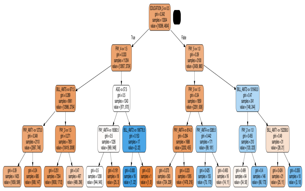
Understanding what hyperparameters are available and the impact of different hyperparameters is a core skill for any data scientist. As models become more complex, there are many different settings you can set, but only some will have a large impact on your model.
You will now assess an existing random forest model (it has some bad choices for hyperparameters!) and then make better choices for a new random forest model and assess its performance.
from sklearn.metrics import confusion_matrix, accuracy_score

rf_clf_old = RandomForestClassifier(min_samples_leaf=1, min_samples_split=2,
                                    n_estimators=5, oob_score=False, random_state=42)

rf_clf_old.fit(X_train, y_train)
rf_old_predictions = rf_clf_old.predict(X_test)

# Print out the old estimator, notice which hyperparameter is badly set
print(rf_clf_old)

# Get confusion matrix & accuracy for the old rf_model
print('Confusion Matrix: \n\n {} \n Accuracy Score: \n\n {}'.format(
    confusion_matrix(y_test, rf_old_predictions),
    accuracy_score(y_test, rf_old_predictions)
))
RandomForestClassifier(n_estimators=5, random_state=42)
Confusion Matrix:
[[6317 693]
[1262 728]]
Accuracy Score:
0.7827777777777778rf_clf_new = RandomForestClassifier(n_estimators=500)
# Fit this to the data and obtain predictions
rf_new_predictions = rf_clf_new.fit(X_train, y_train).predict(X_test)
# Assess the new model (using new predictions!)
print('Confusion Matrix: \n\n', confusion_matrix(y_test, rf_new_predictions))
print('Accuracy Score: \n\n', accuracy_score(y_test, rf_new_predictions))Confusion Matrix:
[[6618 392]
[1274 716]]
Accuracy Score:
0.8148888888888889To apply the concepts learned in the prior exercise, it is good practice to try out learnings on a new algorithm. The k-nearest-neighbors algorithm is not as popular as it used to be but can still be an excellent choice for data that has groups of data that behave similarly. Could this be the case for our credit card users?
In this case you will try out several different values for one of the core hyperparameters for the knn algorithm and compare performance.
from sklearn.neighbors import KNeighborsClassifier

# Build a knn estimator for each value of n_neighbors
knn_5 = KNeighborsClassifier(n_neighbors=5)
knn_10 = KNeighborsClassifier(n_neighbors=10)
knn_20 = KNeighborsClassifier(n_neighbors=20)

# Fit each to the training data & produce predictions
knn_5_predictions = knn_5.fit(X_train, y_train).predict(X_test)
knn_10_predictions = knn_10.fit(X_train, y_train).predict(X_test)
knn_20_predictions = knn_20.fit(X_train, y_train).predict(X_test)

# Get an accuracy score for each of the models
knn_5_accuracy = accuracy_score(y_test, knn_5_predictions)
knn_10_accuracy = accuracy_score(y_test, knn_10_predictions)
knn_20_accuracy = accuracy_score(y_test, knn_20_predictions)
print('The accuracy of 5, 10, 20 neighbors was {}, {}, {}'.format(knn_5_accuracy,
                                                                  knn_10_accuracy,
                                                                  knn_20_accuracy))
The accuracy of 5, 10, 20 neighbors was 0.7508888888888889, 0.7733333333333333, 0.7748888888888888Finding the best hyperparameter of interest without writing hundreds of lines of code for hundreds of models is an important efficiency gain that will greatly assist your future machine learning model building.
An important hyperparameter for the GBM algorithm is the learning rate. But which learning rate is best for this problem? By writing a loop to search through a number of possibilities, collating these and viewing them you can find the best one.
Possible learning rates to try include 0.001, 0.01, 0.05, 0.1, 0.2 and 0.5
from sklearn.ensemble import GradientBoostingClassifier

# Set the learning rates & results storage
learning_rates = [0.001, 0.01, 0.05, 0.1, 0.2, 0.5]
results_list = []

# Create the for loop to evaluate model predictions for each learning rate
for learning_rate in learning_rates:
    model = GradientBoostingClassifier(learning_rate=learning_rate)
    predictions = model.fit(X_train, y_train).predict(X_test)

    # Save the learning rate and accuracy score
    results_list.append([learning_rate, accuracy_score(y_test, predictions)])

# Gather everything into a DataFrame
results_df = pd.DataFrame(results_list, columns=['learning_rate', 'accuracy'])
print(results_df)
learning_rate accuracy
0 0.001 0.778889
1 0.010 0.820000
2 0.050 0.822667
3 0.100 0.821778
4 0.200 0.820333
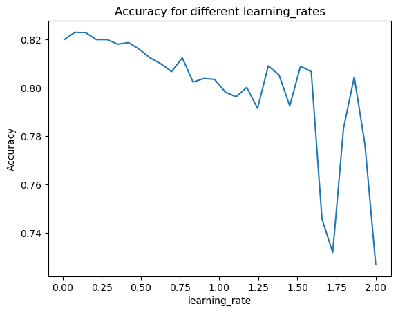
5 0.500 0.813667If we want to test many different values for a single hyperparameter it can be difficult to easily view that in the form of a DataFrame. Previously you learned about a nice trick to analyze this. A graph called a ‘learning curve’ can nicely demonstrate the effect of increasing or decreasing a particular hyperparameter on the final result.
Instead of testing only a few values for the learning rate, you will test many to easily see the effect of this hyperparameter across a large range of values. A useful function from NumPy is np.linspace(start, end, num) which allows you to create a number of values (num) evenly spread within an interval (start, end) that you specify.
learn_rates = np.linspace(0.01, 2, num=30)
accuracies = []

# Create the for loop
for learn_rate in learn_rates:
    # Create the model, predictions & save the accuracies as before
    model = GradientBoostingClassifier(learning_rate=learn_rate)
    predictions = model.fit(X_train, y_train).predict(X_test)
    accuracies.append(accuracy_score(y_test, predictions))

# Plot results
plt.plot(learn_rates, accuracies);
plt.gca().set(xlabel='learning_rate', ylabel='Accuracy', title='Accuracy for different learning_rates');