Code
import numpy as np
import pandas as pd
import tensorflow as tf
import matplotlib.pyplot as plt

plt.rcParams['figure.figsize'] = (8, 8)There will be a discussion on some basic NLP concepts, such as word tokenization and regular expressions for parsing text. We will also cover how to handle non-English texts, as well as more difficult tokenization problems.
This Fine-tuning keras models is part of [Datacamp course: Introduction to Deep Learning in Python] In a wide range of fields such as robotics, natural language processing, image recognition, and artificial intelligence, including AlphaGo, deep learning is the technique behind the most exciting capabilities. As part of this course, you will gain hands-on, practical experience using deep learning with Keras 2.0, the latest version of a cutting-edge Python library for deep learning.
This is my learning experience of data science through DataCamp. These repository contributions are part of my learning journey through my graduate program masters of applied data sciences (MADS) at University Of Michigan, DeepLearning.AI, Coursera & DataCamp. You can find my similar articles & more stories at my medium & LinkedIn profile. I am available at kaggle & github blogs & github repos. Thank you for your motivation, support & valuable feedback.
These include projects, coursework & notebook which I learned through my data science journey. They are created for reproducible & future reference purpose only. All source code, slides or screenshot are intellactual property of respective content authors. If you find these contents beneficial, kindly consider learning subscription from DeepLearning.AI Subscription, Coursera, DataCamp
import numpy as np
import pandas as pd
import tensorflow as tf
import matplotlib.pyplot as plt
plt.rcParams['figure.figsize'] = (8, 8)Now is the time to get your hands dirty with optimization. As a next step, you will optimize a model with a very low learning rate, a very high learning rate, and a “just right” learning rate. Upon completing this exercise, you should review the results, keeping in mind that a low loss function is desirable.
df = pd.read_csv('dataset/titanic_all_numeric.csv')
df.head()| survived | pclass | age | sibsp | parch | fare | male | age_was_missing | embarked_from_cherbourg | embarked_from_queenstown | embarked_from_southampton | |
|---|---|---|---|---|---|---|---|---|---|---|---|
| 0 | 0 | 3 | 22.0 | 1 | 0 | 7.2500 | 1 | False | 0 | 0 | 1 |
| 1 | 1 | 1 | 38.0 | 1 | 0 | 71.2833 | 0 | False | 1 | 0 | 0 |
| 2 | 1 | 3 | 26.0 | 0 | 0 | 7.9250 | 0 | False | 0 | 0 | 1 |
| 3 | 1 | 1 | 35.0 | 1 | 0 | 53.1000 | 0 | False | 0 | 0 | 1 |
| 4 | 0 | 3 | 35.0 | 0 | 0 | 8.0500 | 1 | False | 0 | 0 | 1 |
from tensorflow.keras.utils import to_categorical

predictors = df.iloc[:, 1:].astype(np.float32).to_numpy()
target = to_categorical(df.iloc[:, 0].astype(np.float32).to_numpy())input_shape = (10, )
def get_new_model(input_shape = input_shape):
model = tf.keras.Sequential()
model.add(tf.keras.layers.Dense(100, activation='relu', input_shape = input_shape))
model.add(tf.keras.layers.Dense(100, activation='relu'))
model.add(tf.keras.layers.Dense(2, activation='softmax'))
return modellr_to_test = [0.000001, 0.01, 1]
# Loop over learning rates
for lr in lr_to_test:
print('\n\nTesting model with learning rate: %f\n' % lr)
# Build new model to test, unaffected by previous models
model = get_new_model()
# Create SGD optimizer with specified learning rate: my_optimizer
my_optimizer = tf.keras.optimizers.SGD(lr=lr)
# Compile the model
model.compile(optimizer=my_optimizer, loss='categorical_crossentropy')
# Fit the model
model.fit(predictors, target, epochs=10)WARNING:absl:At this time, the v2.11+ optimizer `tf.keras.optimizers.SGD` runs slowly on M1/M2 Macs, please use the legacy Keras optimizer instead, located at `tf.keras.optimizers.legacy.SGD`.
WARNING:absl:`lr` is deprecated in Keras optimizer, please use `learning_rate` or use the legacy optimizer, e.g.,tf.keras.optimizers.legacy.SGD.
WARNING:absl:There is a known slowdown when using v2.11+ Keras optimizers on M1/M2 Macs. Falling back to the legacy Keras optimizer, i.e., `tf.keras.optimizers.legacy.SGD`.
WARNING:absl:At this time, the v2.11+ optimizer `tf.keras.optimizers.SGD` runs slowly on M1/M2 Macs, please use the legacy Keras optimizer instead, located at `tf.keras.optimizers.legacy.SGD`.
WARNING:absl:`lr` is deprecated in Keras optimizer, please use `learning_rate` or use the legacy optimizer, e.g.,tf.keras.optimizers.legacy.SGD.
WARNING:absl:There is a known slowdown when using v2.11+ Keras optimizers on M1/M2 Macs. Falling back to the legacy Keras optimizer, i.e., `tf.keras.optimizers.legacy.SGD`.
Testing model with learning rate: 0.000001

Epoch 1/10
28/28 [==============================] - 0s 7ms/step - loss: 1.7475
Epoch 2/10
28/28 [==============================] - 0s 6ms/step - loss: 0.6611
Epoch 3/10
28/28 [==============================] - 0s 7ms/step - loss: 0.6218
Epoch 4/10
28/28 [==============================] - 0s 6ms/step - loss: 0.6160
Epoch 5/10
28/28 [==============================] - 0s 6ms/step - loss: 0.6219
Epoch 6/10
28/28 [==============================] - 0s 6ms/step - loss: 0.6221
Epoch 7/10
28/28 [==============================] - 0s 6ms/step - loss: 0.5972
Epoch 8/10
28/28 [==============================] - 0s 6ms/step - loss: 0.6122
Epoch 9/10
28/28 [==============================] - 0s 6ms/step - loss: 0.5872
Epoch 10/10
28/28 [==============================] - 0s 6ms/step - loss: 0.6101


Testing model with learning rate: 0.010000

Epoch 1/10
28/28 [==============================] - 0s 7ms/step - loss: 1.3687
Epoch 2/10
28/28 [==============================] - 0s 6ms/step - loss: 0.6640
Epoch 3/10
28/28 [==============================] - 0s 6ms/step - loss: 0.6407
Epoch 4/10
28/28 [==============================] - 0s 6ms/step - loss: 0.6024
Epoch 5/10
28/28 [==============================] - 0s 6ms/step - loss: 0.5949
Epoch 6/10
28/28 [==============================] - 0s 6ms/step - loss: 0.5895
Epoch 7/10
28/28 [==============================] - 0s 6ms/step - loss: 0.5998
Epoch 8/10
28/28 [==============================] - 0s 6ms/step - loss: 0.5966
Epoch 9/10
28/28 [==============================] - 0s 6ms/step - loss: 0.5847
Epoch 10/10
28/28 [==============================] - 0s 6ms/step - loss: 0.5800


Testing model with learning rate: 1.000000

Epoch 1/10
28/28 [==============================] - 1s 7ms/step - loss: 1.8756
Epoch 2/10
28/28 [==============================] - 0s 6ms/step - loss: 0.6488
Epoch 3/10
28/28 [==============================] - 0s 6ms/step - loss: 0.6314
Epoch 4/10
28/28 [==============================] - 0s 7ms/step - loss: 0.6189
Epoch 5/10
28/28 [==============================] - 0s 6ms/step - loss: 0.6079
Epoch 6/10
28/28 [==============================] - 0s 6ms/step - loss: 0.6083
Epoch 7/10
28/28 [==============================] - 0s 6ms/step - loss: 0.6033
Epoch 8/10
28/28 [==============================] - 0s 6ms/step - loss: 0.6032
Epoch 9/10
28/28 [==============================] - 0s 6ms/step - loss: 0.5889
Epoch 10/10
28/28 [==============================] - 0s 6ms/step - loss: 0.5899Now it’s your turn to monitor model accuracy with a validation data set. A model definition has been provided as model. Your job is to add the code to compile it and then fit it. You’ll check the validation score in each epoch.
n_cols = predictors.shape[1]
input_shape = (n_cols, )

# Specify the model
model = tf.keras.Sequential()
model.add(tf.keras.layers.Dense(100, activation='relu', input_shape=input_shape))
model.add(tf.keras.layers.Dense(100, activation='relu'))
model.add(tf.keras.layers.Dense(2, activation='softmax'))

# Compile the model
model.compile(optimizer='adam', loss='categorical_crossentropy', metrics=['accuracy'])

# Fit the model
hist = model.fit(predictors, target, epochs=10, validation_split=0.3)
Epoch 1/10
20/20 [==============================] - 1s 18ms/step - loss: 0.8775 - accuracy: 0.6324 - val_loss: 0.6027 - val_accuracy: 0.6866
Epoch 2/10
20/20 [==============================] - 0s 11ms/step - loss: 0.7324 - accuracy: 0.6501 - val_loss: 0.5652 - val_accuracy: 0.7276
Epoch 3/10
20/20 [==============================] - 0s 11ms/step - loss: 0.6614 - accuracy: 0.6453 - val_loss: 0.5577 - val_accuracy: 0.7463
Epoch 4/10
20/20 [==============================] - 0s 11ms/step - loss: 0.6296 - accuracy: 0.6709 - val_loss: 0.5096 - val_accuracy: 0.7500
Epoch 5/10
20/20 [==============================] - 0s 11ms/step - loss: 0.6118 - accuracy: 0.6774 - val_loss: 0.4926 - val_accuracy: 0.7537
Epoch 6/10
20/20 [==============================] - 0s 11ms/step - loss: 0.5969 - accuracy: 0.6934 - val_loss: 0.5922 - val_accuracy: 0.7500
Epoch 7/10
20/20 [==============================] - 0s 11ms/step - loss: 0.6406 - accuracy: 0.6918 - val_loss: 0.5396 - val_accuracy: 0.7201
Epoch 8/10
20/20 [==============================] - 0s 11ms/step - loss: 0.5769 - accuracy: 0.7030 - val_loss: 0.5332 - val_accuracy: 0.7873
Epoch 9/10
20/20 [==============================] - 0s 11ms/step - loss: 0.5775 - accuracy: 0.7175 - val_loss: 0.5964 - val_accuracy: 0.6866
Epoch 10/10
20/20 [==============================] - 0s 11ms/step - loss: 0.6409 - accuracy: 0.7271 - val_loss: 0.5226 - val_accuracy: 0.7873Now that you know how to monitor your model performance throughout optimization, you can use early stopping to stop optimization when it isn’t helping any more. Since the optimization stops automatically when it isn’t helping, you can also set a high value for epochs in your call to .fit().
from tensorflow.keras.callbacks import EarlyStopping

# Save the number of columns in predictors: n_cols
n_cols = predictors.shape[1]
input_shape = (n_cols, )

# Specify the model
model = tf.keras.Sequential()
model.add(tf.keras.layers.Dense(100, activation='relu', input_shape=input_shape))
model.add(tf.keras.layers.Dense(100, activation='relu'))
model.add(tf.keras.layers.Dense(2, activation='softmax'))

# Compile the model
model.compile(optimizer='adam', loss='categorical_crossentropy', metrics=['accuracy'])

# Define early_stopping_monitor
early_stopping_monitor = EarlyStopping(patience=2)

# Fit the model
model.fit(predictors, target, epochs=30, validation_split=0.3,
          callbacks=[early_stopping_monitor])

print("\nBecause optimization will automatically stop when it is no longer helpful, it is okay to specify the maximum number of epochs as 30 rather than using the default of 10 that you've used so far. Here, it seems like the optimization stopped after 4 epochs.")
Epoch 1/30
20/20 [==============================] - 1s 17ms/step - loss: 0.7307 - accuracy: 0.6132 - val_loss: 0.6820 - val_accuracy: 0.6940
Epoch 2/30
20/20 [==============================] - 0s 11ms/step - loss: 0.6902 - accuracy: 0.6404 - val_loss: 0.5921 - val_accuracy: 0.7239
Epoch 3/30
20/20 [==============================] - 0s 11ms/step - loss: 0.6624 - accuracy: 0.6677 - val_loss: 0.5234 - val_accuracy: 0.7351
Epoch 4/30
20/20 [==============================] - 0s 11ms/step - loss: 0.6245 - accuracy: 0.6950 - val_loss: 0.5368 - val_accuracy: 0.7313
Epoch 5/30
20/20 [==============================] - 0s 11ms/step - loss: 0.6476 - accuracy: 0.6758 - val_loss: 0.5154 - val_accuracy: 0.7612
Epoch 6/30
20/20 [==============================] - 0s 11ms/step - loss: 0.6226 - accuracy: 0.6774 - val_loss: 0.5410 - val_accuracy: 0.7724
Epoch 7/30
20/20 [==============================] - 0s 11ms/step - loss: 0.6440 - accuracy: 0.6950 - val_loss: 0.6073 - val_accuracy: 0.6903
Because optimization will automatically stop when it is no longer helpful, it is okay to specify the maximum number of epochs as 30 rather than using the default of 10 that you've used so far. Here, it seems like the optimization stopped after 4 epochs.You now have all the information you need to begin experimenting with different models.
Pre-loaded is a model named model_1. It is a relatively small network, with only ten units in each hidden layer.
As part of this exercise, you will create a new model called model_2 which is similar to model_1, except that it has 100 units in each hidden layer.
As soon as model_2 is created, both models will be fitted, and a graph will be displayed showing each model’s loss score at each epoch. We have added the argument verbose=False to the fitting commands in order to print out fewer updates since they will be displayed graphically rather than as text.
After you hit run, the outputs will take a moment to appear because you are fitting two models.
model_1 = tf.keras.Sequential()
model_1.add(tf.keras.layers.Dense(10, activation='relu', input_shape=input_shape))
model_1.add(tf.keras.layers.Dense(10, activation='relu'))
model_1.add(tf.keras.layers.Dense(2, activation='softmax'))
model_1.compile(optimizer='adam', loss='categorical_crossentropy', metrics=['accuracy'])model_1.summary()Model: "sequential_15"
_________________________________________________________________
Layer (type) Output Shape Param #
=================================================================
dense_45 (Dense) (None, 10) 110
dense_46 (Dense) (None, 10) 110
dense_47 (Dense) (None, 2) 22
=================================================================
Total params: 242
Trainable params: 242
Non-trainable params: 0
_________________________________________________________________early_stopping_monitor = EarlyStopping(patience=2)
# Create the new model: model_2
model_2 = tf.keras.Sequential()
# Add the first and second layers
model_2.add(tf.keras.layers.Dense(100, activation='relu', input_shape=input_shape))
model_2.add(tf.keras.layers.Dense(100, activation='relu'))
# Add the output layer
model_2.add(tf.keras.layers.Dense(2, activation='softmax'))
# Compile model_2
model_2.compile(optimizer='adam', loss='categorical_crossentropy', metrics=['accuracy'])
# Fit model_1
model_1_training = model_1.fit(predictors, target, epochs=15, validation_split=0.2,
callbacks=[early_stopping_monitor], verbose=False)
# Fit model_2
model_2_training = model_2.fit(predictors, target, epochs=15, validation_split=0.2,
callbacks=[early_stopping_monitor], verbose=False)
# Create th eplot
plt.plot(model_1_training.history['val_loss'], 'r', model_2_training.history['val_loss'], 'b');
plt.xlabel('Epochs')
plt.ylabel('Validation score');
print("\nThe blue model is the one you made, the red is the original model. Your model had a lower loss value, so it is the better model")
The blue model is the one you made, the red is the original model. Your model had a lower loss value, so it is the better model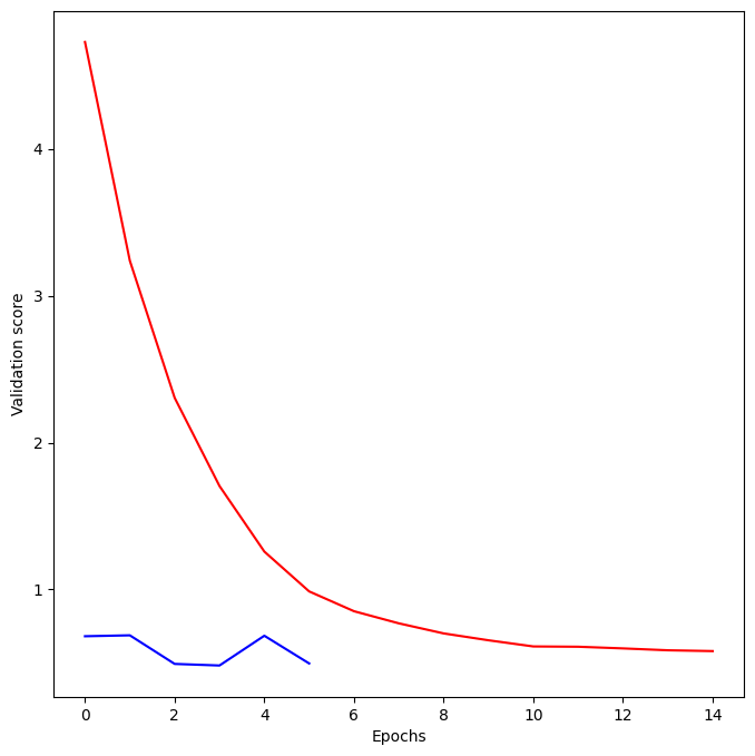
You’ve seen how to experiment with wider networks. In this exercise, you’ll try a deeper network (more hidden layers).
Once again, you have a baseline model called model_1 as a starting point. It has 1 hidden layer, with 50 units. You can see a summary of that model’s structure printed out. You will create a similar network with 3 hidden layers (still keeping 50 units in each layer).
This will again take a moment to fit both models, so you’ll need to wait a few seconds to see the results after you run your code.
model_1 = tf.keras.Sequential()
model_1.add(tf.keras.layers.Dense(50, activation='relu', input_shape=input_shape))
model_1.add(tf.keras.layers.Dense(2, activation='softmax'))
model_1.compile(optimizer='adam', loss='categorical_crossentropy', metrics=['accuracy'])model_1.summary()Model: "sequential_17"
_________________________________________________________________
Layer (type) Output Shape Param #
=================================================================
dense_51 (Dense) (None, 50) 550
dense_52 (Dense) (None, 2) 102
=================================================================
Total params: 652
Trainable params: 652
Non-trainable params: 0
_________________________________________________________________model_2 = tf.keras.Sequential()
# Add the first, second, and third hidden layers
model_2.add(tf.keras.layers.Dense(50, activation='relu', input_shape=input_shape))
model_2.add(tf.keras.layers.Dense(50, activation='relu'))
model_2.add(tf.keras.layers.Dense(50, activation='relu'))
# Add the output layer
model_2.add(tf.keras.layers.Dense(2, activation='softmax'))
# Compile model_2
model_2.compile(optimizer='adam', loss='categorical_crossentropy', metrics=['accuracy'])
# Fit model 1
model_1_training = model_1.fit(predictors, target, epochs=20, validation_split=0.4, callbacks=[early_stopping_monitor], verbose=False)
# Fit model 2
model_2_training = model_2.fit(predictors, target, epochs=20, validation_split=0.4, callbacks=[early_stopping_monitor], verbose=False)
# Create the plot
plt.plot(model_1_training.history['val_loss'], 'r', model_2_training.history['val_loss'], 'b');
plt.xlabel('Epochs');
plt.ylabel('Validation score');
print("\nThe blue model is the one you made and the red is the original model. The model with the lower loss value is the better model")
The blue model is the one you made and the red is the original model. The model with the lower loss value is the better model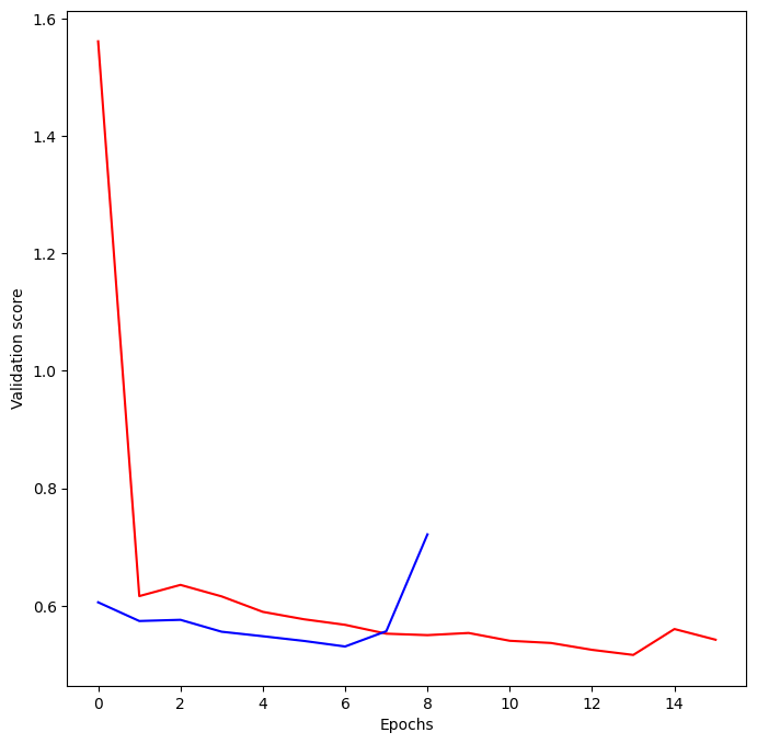
You’ve reached the final exercise of the course - you now know everything you need to build an accurate model to recognize handwritten digits!
To add an extra challenge, we’ve loaded only 2500 images, rather than 60000 which you will see in some published results. Deep learning models perform better with more data, however, they also take longer to train, especially when they start becoming more complex.
If you have a computer with a CUDA compatible GPU, you can take advantage of it to improve computation time. If you don’t have a GPU, no problem! You can set up a deep learning environment in the cloud that can run your models on a GPU. Here is a blog post by Dan that explains how to do this - check it out after completing this exercise! It is a great next step as you continue your deep learning journey.
mnist = pd.read_csv('dataset/mnist.csv', header=None)
mnist.head()| 0 | 1 | 2 | 3 | 4 | 5 | 6 | 7 | 8 | 9 | ... | 775 | 776 | 777 | 778 | 779 | 780 | 781 | 782 | 783 | 784 | |
|---|---|---|---|---|---|---|---|---|---|---|---|---|---|---|---|---|---|---|---|---|---|
| 0 | 5 | 0 | 0.1 | 0.2 | 0.3 | 0.4 | 0.5 | 0.6 | 0.7 | 0.8 | ... | 0.608 | 0.609 | 0.61 | 0.611 | 0.612 | 0.613 | 0.614 | 0.615 | 0.616 | 0.617 |
| 1 | 4 | 0 | 0.0 | 0.0 | 0.0 | 0.0 | 0.0 | 0.0 | 0.0 | 0.0 | ... | 0.000 | 0.000 | 0.00 | 0.000 | 0.000 | 0.000 | 0.000 | 0.000 | 0.000 | 0.000 |
| 2 | 3 | 0 | 0.0 | 0.0 | 0.0 | 0.0 | 0.0 | 0.0 | 0.0 | 0.0 | ... | 0.000 | 0.000 | 0.00 | 0.000 | 0.000 | 0.000 | 0.000 | 0.000 | 0.000 | 0.000 |
| 3 | 0 | 0 | 0.0 | 0.0 | 0.0 | 0.0 | 0.0 | 0.0 | 0.0 | 0.0 | ... | 0.000 | 0.000 | 0.00 | 0.000 | 0.000 | 0.000 | 0.000 | 0.000 | 0.000 | 0.000 |
| 4 | 2 | 0 | 0.0 | 0.0 | 0.0 | 0.0 | 0.0 | 0.0 | 0.0 | 0.0 | ... | 0.000 | 0.000 | 0.00 | 0.000 | 0.000 | 0.000 | 0.000 | 0.000 | 0.000 | 0.000 |
5 rows × 785 columns
X = mnist.iloc[:, 1:].astype(np.float32).to_numpy()
y = to_categorical(mnist.iloc[:, 0])model = tf.keras.Sequential()
# Add the first hidden layer
model.add(tf.keras.layers.Dense(50, activation='relu', input_shape=(X.shape[1], )))
# Add the second hidden layer
model.add(tf.keras.layers.Dense(50, activation='relu'))
# Add the output layer
model.add(tf.keras.layers.Dense(10, activation='softmax'))
# Compile the model
model.compile(optimizer='adam', loss='categorical_crossentropy', metrics=['accuracy'])
# Fit the model
model.fit(X, y, validation_split=0.3, epochs=50);Epoch 1/50
44/44 [==============================] - 1s 16ms/step - loss: 24.8658 - accuracy: 0.4379 - val_loss: 8.2308 - val_accuracy: 0.6106
Epoch 2/50
44/44 [==============================] - 1s 12ms/step - loss: 4.4352 - accuracy: 0.7250 - val_loss: 5.0027 - val_accuracy: 0.7088
Epoch 3/50
44/44 [==============================] - 0s 11ms/step - loss: 2.2376 - accuracy: 0.8264 - val_loss: 4.1121 - val_accuracy: 0.7354
Epoch 4/50
44/44 [==============================] - 0s 11ms/step - loss: 1.2230 - accuracy: 0.8843 - val_loss: 4.0306 - val_accuracy: 0.7255
Epoch 5/50
44/44 [==============================] - 0s 11ms/step - loss: 0.7398 - accuracy: 0.8993 - val_loss: 3.6222 - val_accuracy: 0.7454
Epoch 6/50
44/44 [==============================] - 0s 11ms/step - loss: 0.4634 - accuracy: 0.9207 - val_loss: 3.5127 - val_accuracy: 0.7421
Epoch 7/50
44/44 [==============================] - 1s 12ms/step - loss: 0.2833 - accuracy: 0.9471 - val_loss: 3.5105 - val_accuracy: 0.7504
Epoch 8/50
44/44 [==============================] - 0s 11ms/step - loss: 0.1764 - accuracy: 0.9614 - val_loss: 3.1653 - val_accuracy: 0.7820
Epoch 9/50
44/44 [==============================] - 0s 11ms/step - loss: 0.1530 - accuracy: 0.9671 - val_loss: 3.0793 - val_accuracy: 0.7804
Epoch 10/50
44/44 [==============================] - 0s 11ms/step - loss: 0.0964 - accuracy: 0.9814 - val_loss: 3.1622 - val_accuracy: 0.7870
Epoch 11/50
44/44 [==============================] - 0s 11ms/step - loss: 0.0619 - accuracy: 0.9821 - val_loss: 3.3843 - val_accuracy: 0.7787
Epoch 12/50
44/44 [==============================] - 0s 11ms/step - loss: 0.1169 - accuracy: 0.9729 - val_loss: 3.3640 - val_accuracy: 0.7704
Epoch 13/50
44/44 [==============================] - 0s 11ms/step - loss: 0.0575 - accuracy: 0.9850 - val_loss: 3.1171 - val_accuracy: 0.7987
Epoch 14/50
44/44 [==============================] - 0s 11ms/step - loss: 0.0164 - accuracy: 0.9936 - val_loss: 3.1772 - val_accuracy: 0.7887
Epoch 15/50
44/44 [==============================] - 1s 13ms/step - loss: 0.0228 - accuracy: 0.9943 - val_loss: 3.0467 - val_accuracy: 0.7837
Epoch 16/50
44/44 [==============================] - 0s 11ms/step - loss: 0.0131 - accuracy: 0.9957 - val_loss: 3.0532 - val_accuracy: 0.7854
Epoch 17/50
44/44 [==============================] - 0s 11ms/step - loss: 0.0091 - accuracy: 0.9971 - val_loss: 2.9317 - val_accuracy: 0.8053
Epoch 18/50
44/44 [==============================] - 0s 11ms/step - loss: 0.0015 - accuracy: 0.9993 - val_loss: 2.9325 - val_accuracy: 0.8037
Epoch 19/50
44/44 [==============================] - 0s 11ms/step - loss: 4.3801e-04 - accuracy: 1.0000 - val_loss: 2.9202 - val_accuracy: 0.8070
Epoch 20/50
44/44 [==============================] - 0s 11ms/step - loss: 2.2381e-04 - accuracy: 1.0000 - val_loss: 2.9102 - val_accuracy: 0.8103
Epoch 21/50
44/44 [==============================] - 0s 11ms/step - loss: 1.8700e-04 - accuracy: 1.0000 - val_loss: 2.9083 - val_accuracy: 0.8153
Epoch 22/50
44/44 [==============================] - 1s 11ms/step - loss: 1.6427e-04 - accuracy: 1.0000 - val_loss: 2.9064 - val_accuracy: 0.8153
Epoch 23/50
44/44 [==============================] - 1s 12ms/step - loss: 1.5058e-04 - accuracy: 1.0000 - val_loss: 2.9043 - val_accuracy: 0.8153
Epoch 24/50
44/44 [==============================] - 0s 11ms/step - loss: 1.3891e-04 - accuracy: 1.0000 - val_loss: 2.9032 - val_accuracy: 0.8170
Epoch 25/50
44/44 [==============================] - 0s 11ms/step - loss: 1.2836e-04 - accuracy: 1.0000 - val_loss: 2.9009 - val_accuracy: 0.8153
Epoch 26/50
44/44 [==============================] - 0s 11ms/step - loss: 1.2056e-04 - accuracy: 1.0000 - val_loss: 2.9005 - val_accuracy: 0.8153
Epoch 27/50
44/44 [==============================] - 0s 11ms/step - loss: 1.1373e-04 - accuracy: 1.0000 - val_loss: 2.8997 - val_accuracy: 0.8170
Epoch 28/50
44/44 [==============================] - 0s 11ms/step - loss: 1.0786e-04 - accuracy: 1.0000 - val_loss: 2.8992 - val_accuracy: 0.8170
Epoch 29/50
44/44 [==============================] - 0s 11ms/step - loss: 1.0281e-04 - accuracy: 1.0000 - val_loss: 2.8984 - val_accuracy: 0.8170
Epoch 30/50
44/44 [==============================] - 0s 11ms/step - loss: 9.7687e-05 - accuracy: 1.0000 - val_loss: 2.8987 - val_accuracy: 0.8170
Epoch 31/50
44/44 [==============================] - 0s 11ms/step - loss: 9.3267e-05 - accuracy: 1.0000 - val_loss: 2.8983 - val_accuracy: 0.8136
Epoch 32/50
44/44 [==============================] - 0s 11ms/step - loss: 8.9666e-05 - accuracy: 1.0000 - val_loss: 2.8974 - val_accuracy: 0.8136
Epoch 33/50
44/44 [==============================] - 0s 10ms/step - loss: 8.6012e-05 - accuracy: 1.0000 - val_loss: 2.8975 - val_accuracy: 0.8136
Epoch 34/50
44/44 [==============================] - 0s 11ms/step - loss: 8.2911e-05 - accuracy: 1.0000 - val_loss: 2.8974 - val_accuracy: 0.8153
Epoch 35/50
44/44 [==============================] - 0s 11ms/step - loss: 7.9426e-05 - accuracy: 1.0000 - val_loss: 2.8968 - val_accuracy: 0.8153
Epoch 36/50
44/44 [==============================] - 0s 11ms/step - loss: 7.6373e-05 - accuracy: 1.0000 - val_loss: 2.8970 - val_accuracy: 0.8136
Epoch 37/50
44/44 [==============================] - 0s 10ms/step - loss: 7.3901e-05 - accuracy: 1.0000 - val_loss: 2.8966 - val_accuracy: 0.8136
Epoch 38/50
44/44 [==============================] - 0s 10ms/step - loss: 7.1073e-05 - accuracy: 1.0000 - val_loss: 2.8970 - val_accuracy: 0.8120
Epoch 39/50
44/44 [==============================] - 0s 10ms/step - loss: 6.8472e-05 - accuracy: 1.0000 - val_loss: 2.8967 - val_accuracy: 0.8120
Epoch 40/50
44/44 [==============================] - 0s 11ms/step - loss: 6.6433e-05 - accuracy: 1.0000 - val_loss: 2.8969 - val_accuracy: 0.8120
Epoch 41/50
44/44 [==============================] - 0s 11ms/step - loss: 6.4350e-05 - accuracy: 1.0000 - val_loss: 2.8965 - val_accuracy: 0.8120
Epoch 42/50
44/44 [==============================] - 1s 12ms/step - loss: 6.2323e-05 - accuracy: 1.0000 - val_loss: 2.8968 - val_accuracy: 0.8120
Epoch 43/50
44/44 [==============================] - 0s 11ms/step - loss: 6.0372e-05 - accuracy: 1.0000 - val_loss: 2.8966 - val_accuracy: 0.8103
Epoch 44/50
44/44 [==============================] - 1s 11ms/step - loss: 5.8557e-05 - accuracy: 1.0000 - val_loss: 2.8969 - val_accuracy: 0.8103
Epoch 45/50
44/44 [==============================] - 0s 11ms/step - loss: 5.6897e-05 - accuracy: 1.0000 - val_loss: 2.8967 - val_accuracy: 0.8103
Epoch 46/50
44/44 [==============================] - 0s 11ms/step - loss: 5.5444e-05 - accuracy: 1.0000 - val_loss: 2.8973 - val_accuracy: 0.8103
Epoch 47/50
44/44 [==============================] - 0s 11ms/step - loss: 5.3896e-05 - accuracy: 1.0000 - val_loss: 2.8972 - val_accuracy: 0.8103
Epoch 48/50
44/44 [==============================] - 0s 11ms/step - loss: 5.2403e-05 - accuracy: 1.0000 - val_loss: 2.8977 - val_accuracy: 0.8103
Epoch 49/50
44/44 [==============================] - 0s 11ms/step - loss: 5.1018e-05 - accuracy: 1.0000 - val_loss: 2.8979 - val_accuracy: 0.8103
Epoch 50/50
44/44 [==============================] - 0s 10ms/step - loss: 4.9726e-05 - accuracy: 1.0000 - val_loss: 2.8983 - val_accuracy: 0.8103print("\nYou've done something pretty amazing. The code you wrote leads to a model that's 90% accurate at recognizing handwritten digits, even while using a small training set of only 1750 images!")
You've done something pretty amazing. The code you wrote leads to a model that's 90% accurate at recognizing handwritten digits, even while using a small training set of only 1750 images!