Back Propagation

python

deep learning.ai

machine learning

supervised learning

back propagation

neural network

Author

kakamana

Published

May 9, 2023

Back Propagation

This describes compute graphs and their use in back propagation. Working through this lab will give you insight into a key algorithm used by most machine learning frameworks. Gradient descent requires the derivative of the cost with respect to each parameter in the network. Neural networks can have millions or even billions of parameters. The back propagation algorithm is used to compute those derivatives. Computation graphs are used to simplify the operation.

This Back Propagation is part of DeepLearning.AI course: Machine Learning Specialization / Course 2: Advanced Learning Algorithms: Back propagation You will build and train a neural network with TensorFlow to perform multi-class classification in the second course of the Machine Learning Specialization. Ensure that your machine learning models are generalizable by applying best practices for machine learning development. You will build and train a neural network using TensorFlow to perform multi-class classification in the second course of the Machine Learning Specialization. Implement best practices for machine learning development to ensure that your models are generalizable to real-world data and tasks. Create and use decision trees and tree ensemble methods, including random forests and boosted trees.

This is my learning experience of data science through DeepLearning.AI. These repository contributions are part of my learning journey through my graduate program masters of applied data sciences (MADS) at University Of Michigan, DeepLearning.AI, Coursera & DataCamp. You can find my similar articles & more stories at my medium & LinkedIn profile. I am available at kaggle & github blogs & github repos. Thank you for your motivation, support & valuable feedback.

These include projects, coursework & notebook which I learned through my data science journey. They are created for reproducible & future reference purpose only. All source code, slides or screenshot are intellectual property of respective content authors. If you find these contents beneficial, kindly consider learning subscription from DeepLearning.AI Subscription, Coursera, DataCamp

Code

from sympy import *
import numpy as np
import re
%matplotlib widget
import matplotlib.pyplot as plt
from matplotlib.widgets import TextBox
from matplotlib.widgets import Button
import ipywidgets as widgets
from lab_utils_backprop import *

Computation Graph

A computation graph simplifies the computation of complex derivatives by breaking them into smaller steps. Let’s see how this works.

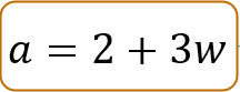
Let’s calculate the derivative of this slightly complex expression, $J = (2+3w)^2$. We would like to find the derivative of $J$ with respect to $w$ or $\frac{\partial J}{\partial w}$.

Code

plt.close("all")
plt_network(config_nw0, "C2_W2_BP_network0.PNG")

<lab_utils_backprop.plt_network at 0x1771b5b7ca0>

Forward Propagation

Let’s calculate the values in the forward direction.

Just a note about this section. It uses global variables and reuses them as the calculation progresses. If you run cells out of order, you may get funny results. If you do, go back to this point and run them in order.

Code

w = 3
a = 2+3*w
J = a**2
print(f"a = {a}, J = {J}")

a = 11, J = 121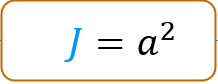

Backprop

Backprop is the algorithm we use to calculate derivatives. As described in the lectures, backprop starts at the right and moves to the left. The first node to consider is $J = a^2 $ and the first step is to find $\frac{\partial J}{\partial a}$

$\frac{\partial J}{\partial a}$

Arithmetically

Find $\frac{\partial J}{\partial a}$ by finding how $J$ changes as a result of a little change in $a$. This is described in detail in the derivatives optional lab.

Code

a_epsilon = a + 0.001       # a epsilon
J_epsilon = a_epsilon**2    # J_epsilon
k = (J_epsilon - J)/0.001   # difference divided by epsilon
print(f"J = {J}, J_epsilon = {J_epsilon}, dJ_da ~= k = {k} ")

J = 121, J_epsilon = 121.02200099999999, dJ_da ~= k = 22.000999999988835

$\frac{\partial J}{\partial a}$ is 22 which is $2\times a$. Our result is not exactly $2 \times a$ because our epsilon value is not infinitesimally small. #### Symbolically Now, let’s use SymPy to calculate derivatives symbolically as we did in the derivatives optional lab. We will prefix the name of the variable with an ‘s’ to indicate this is a symbolic variable.

Code

sw,sJ,sa = symbols('w,J,a')
sJ = sa**2
sJ

a**2

Code

sJ.subs([(sa,a)])

Code

dJ_da = diff(sJ, sa)
dJ_da

2*a

So, $\frac{\partial J}{\partial a} = 2a$. When $a=11$, $\frac{\partial J}{\partial a} = 22$. This matches our arithmetic calculation above. If you have not already done so, you can go back to the diagram above and fill in the value for $\frac{\partial J}{\partial a}$.

$\frac{\partial J}{\partial w}$

Moving from right to left, the next value we would like to compute is $\frac{\partial J}{\partial w}$. To do this, we first need to calculate $\frac{\partial a}{\partial w}$ which describes how the output of this node, $a$, changes when the input $w$ changes a little bit.

Arithmetically

Find $\frac{\partial a}{\partial w}$ by finding how $a$ changes as a result of a little change in $w$.

Calculated arithmetically, $\frac{\partial a}{\partial w} \approx 3$. Let’s try it with SymPy.

Code

sa = 2 + 3*sw
sa

3*w + 2

Code

da_dw = diff(sa,sw)
da_dw

The next step is the interesting part: - We know that a small change in $w$ will cause $a$ to change by 3 times that amount. - We know that a small change in $a$ will cause $J$ to change by $2\times a$ times that amount. (a=11 in this example) so, putting these together, - We know that a small change in $w$ will cause $J$ to change by $3 \times 2\times a$ times that amount.

These cascading changes go by the name of the chain rule. It can be written like this: \[\frac{\partial J}{\partial w} = \frac{\partial a}{\partial w} \frac{\partial J}{\partial a} \]

It’s worth spending some time thinking this through if it is not clear. This is a key take-away.

Let’s try calculating it:

Code

dJ_dw = da_dw * dJ_da
dJ_dw

6*a

And $a$ is 11 in this example so $\frac{\partial J}{\partial w} = 66$. We can check this arithmetically:

Code

w_epsilon = w + 0.001
a_epsilon = 2 + 3*w_epsilon
J_epsilon = a_epsilon**2
k = (J_epsilon - J)/0.001   # difference divided by epsilon
print(f"J = {J}, J_epsilon = {J_epsilon}, dJ_dw ~= k = {k} ")

J = 121, J_epsilon = 121.06600900000001, dJ_dw ~= k = 66.0090000000082

Another view One could visualize these cascading changes this way: 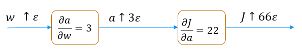A small change in $w$ is multiplied by $\frac{\partial a}{\partial w}$ resulting in a change that is 3 times as large. This larger change is then multiplied by $\frac{\partial J}{\partial a}$ resulting in a change that is now $3 \times 22 = 66$ times larger.

Computation Graph of a Simple Neural Network

Below is a graph of the neural network used in the lecture with different values. Try and fill in the values in the boxes. Note, the interactive graphic is not particularly robust. If you run into trouble with the interface, run the cell below again to restart.

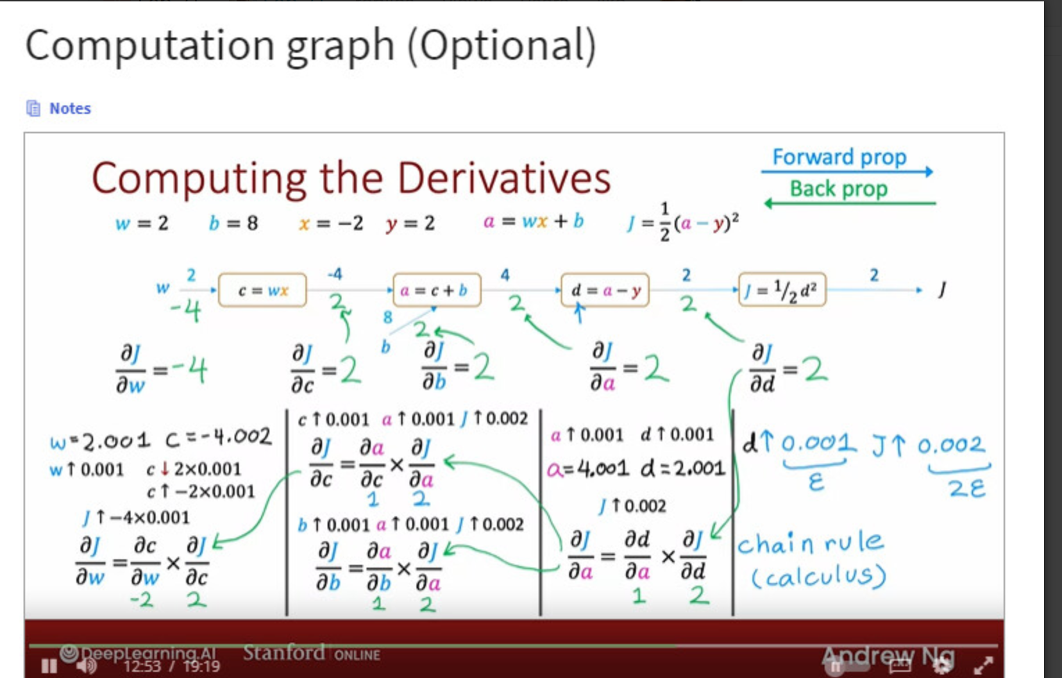
Below, we will go through the computations required to fill in the above computation graph in detail. We start with the forward path.

Forward propagation

The calculations in the forward path are the ones you have recently learned for neural networks. You can compare the values below to those you calculated for the diagram above.

Code

# Inputs and parameters
x = 2
w = -2
b = 8
y = 1
# calculate per step values
c = w * x
a = c + b
d = a - y
J = d**2/2
print(f"J={J}, d={d}, a={a}, c={c}")

J=4.5, d=3, a=4, c=-4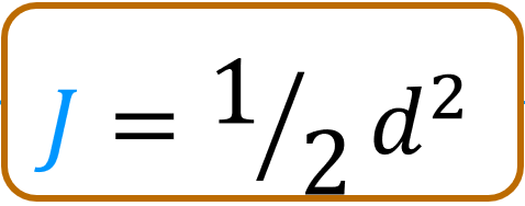

Backward propagation (Backprop)

As described in the lectures, backprop starts at the right and moves to the left. The first node to consider is $J = d^2 $ and the first step is to find $\frac{\partial J}{\partial d}$

$\frac{\partial J}{\partial d}$

Arithmetically

Find $\frac{\partial J}{\partial d}$ by finding how $J$ changes as a result of a little change in $d$.

Code

d_epsilon = d + 0.001
J_epsilon = d_epsilon**2/2
k = (J_epsilon - J)/0.001   # difference divided by epsilon
print(f"J = {J}, J_epsilon = {J_epsilon}, dJ_dd ~= k = {k} ")

J = 4.5, J_epsilon = 4.5030005, dJ_dd ~= k = 3.0004999999997395

$\frac{\partial J}{\partial d}$ is 3, which is the value of $d$. Our result is not exactly $d$ because our epsilon value is not infinitesimally small. #### Symbolically Now, let’s use SymPy to calculate derivatives symbolically, as we did in the derivatives optional lab. We will prefix the name of the variable with an ‘s’ to indicate this is a symbolic variable.

Code

sx,sw,sb,sy,sJ = symbols('x,w,b,y,J')
sa, sc, sd = symbols('a,c,d')
sJ = sd**2/2
sJ

d**2/2

Code

sJ.subs([(sd,d)])

9/2

Code

dJ_dd = diff(sJ, sd)
dJ_dd

So, $\frac{\partial J}{\partial d}$ = d. When $d=3$, $\frac{\partial J}{\partial d}$ = 3. This matches our arithmetic calculation above. If you have not already done so, you can go back to the diagram above and fill in the value for $\frac{\partial J}{\partial d}$.

$\frac{\partial J}{\partial a}$

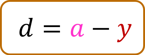Moving from right to left, the next value we would like to compute is $\frac{\partial J}{\partial a}$. To do this, we first need to calculate $\frac{\partial d}{\partial a}$ which describes how the output of this node changes when the input $a$ changes a little bit. (Note, we are not interested in how the output changes when $y$ changes since $y$ is not a parameter.)

Arithmetically

Find $\frac{\partial d}{\partial a}$ by finding how $d$ changes as a result of a little change in $a$.

Code

a_epsilon = a + 0.001         # a  plus a small value
d_epsilon = a_epsilon - y
k = (d_epsilon - d)/0.001   # difference divided by epsilon
print(f"d = {d}, d_epsilon = {d_epsilon}, dd_da ~= k = {k} ")

d = 3, d_epsilon = 3.0010000000000003, dd_da ~= k = 1.000000000000334

Calculated arithmetically, $\frac{\partial d}{\partial a} \approx 1$. Let’s try it with SymPy. #### Symbolically

Code

sd = sa - sy
sd

a - y

Code

dd_da = diff(sd,sa)
dd_da

Calculated arithmetically, $\frac{\partial d}{\partial a}$ also equals 1. >The next step is the interesting part, repeated again in this example: > - We know that a small change in $a$ will cause $d$ to change by 1 times that amount. > - We know that a small change in $d$ will cause $J$ to change by $d$ times that amount. (d=3 in this example) so, putting these together, > - We know that a small change in $a$ will cause $J$ to change by $1\times d$ times that amount. > >This is again the chain rule. It can be written like this: \[\frac{\partial J}{\partial a} = \frac{\partial d}{\partial a} \frac{\partial J}{\partial d} \]

Let’s try calculating it:

Code

dJ_da = dd_da * dJ_dd
dJ_da

And $d$ is 3 in this example so $\frac{\partial J}{\partial a} = 3$. We can check this arithmetically:

Code

a_epsilon = a + 0.001
d_epsilon = a_epsilon - y
J_epsilon = d_epsilon**2/2
k = (J_epsilon - J)/0.001
print(f"J = {J}, J_epsilon = {J_epsilon}, dJ_da ~= k = {k} ")

J = 4.5, J_epsilon = 4.503000500000001, dJ_da ~= k = 3.0005000000006277

OK, they match! You can now fill the values for $\frac{\partial d}{\partial a}$ and $\frac{\partial J}{\partial a}$ in the diagram if you have not already done so.

The steps in backprop Now that you have worked through several nodes, we can write down the basic method:
working right to left, for each node: - calculate the local derivative(s) of the node - using the chain rule, combine with the derivative of the cost with respect to the node to the right.

The ‘local derivative(s)’ are the derivative(s) of the output of the current node with respect to all inputs or parameters.

Let’s continue the job. We’ll be a bit less verbose now that you are familiar with the method.

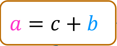$\frac{\partial J}{\partial c}$, $\frac{\partial J}{\partial b}$

The next node has two derivatives of interest. We need to calculate $\frac{\partial J}{\partial c}$ so we can propagate to the left. We also want to calculate $\frac{\partial J}{\partial b}$. Finding the derivative of the cost with respect to the parameters $w$ and $b$ is the object of backprop. We will find the local derivatives, $\frac{\partial a}{\partial c}$ and $\frac{\partial a}{\partial b}$ first and then combine those with the derivative coming from the right, $\frac{\partial J}{\partial a}$.

Code

# calculate the local derivatives da_dc, da_db
sa = sc + sb
sa

b + c

Code

da_dc = diff(sa,sc)
da_db = diff(sa,sb)
print(da_dc, da_db)

1 1

Code

dJ_dc = da_dc * dJ_da
dJ_db = da_db * dJ_da
print(f"dJ_dc = {dJ_dc},  dJ_db = {dJ_db}")

dJ_dc = d,  dJ_db = d

And in our example, d = 3

$\frac{\partial J}{\partial w}$

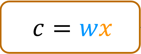The last node in this example calculates c. Here, we are interested in how J changes with respect to the parameter w. We will not back propagate to the input $x$, so we are not interested in $\frac{\partial J}{\partial x}$. Let’s start by calculating $\frac{\partial c}{\partial w}$.

Code

# calculate the local derivative
sc = sw * sx
sc

w*x

Code

dc_dw = diff(sc,sw)
dc_dw

This derivative is a bit more exciting than the last one. This will vary depending on the value of $x$. This is 2 in our example.

Combine this with $\frac{\partial J}{\partial c}$ to find $\frac{\partial J}{\partial w}$.

Code

dJ_dw = dc_dw * dJ_dc
dJ_dw

d*x

Code

print(f"dJ_dw = {dJ_dw.subs([(sd,d),(sx,x)])}")

dJ_dw = 2*d

$d=3$, so $\frac{\partial J}{\partial w} = 6$ for our example. Let’s test this arithmetically:

Code

J_epsilon = ((w+0.001)*x+b - y)**2/2
k = (J_epsilon - J)/0.001
print(f"J = {J}, J_epsilon = {J_epsilon}, dJ_dw ~= k = {k} ")

J = 4.5, J_epsilon = 4.506002, dJ_dw ~= k = 6.001999999999619

Back Propagation

Back Propagation

Computation Graph

Forward Propagation

Backprop

\(\frac{\partial J}{\partial a}\)

Arithmetically

\(\frac{\partial J}{\partial w}\)

Arithmetically

Computation Graph of a Simple Neural Network

Forward propagation

Backward propagation (Backprop)

\(\frac{\partial J}{\partial d}\)

Arithmetically

\(\frac{\partial J}{\partial a}\)

Arithmetically

\(\frac{\partial J}{\partial c}\), \(\frac{\partial J}{\partial b}\)

\(\frac{\partial J}{\partial w}\)